Table of Contents
Introduction
There are many instances where calibration frames do not properly calibrate an image or where time or conditions do not afford the opportunity of taking them. In many cases the resulting vignetting and gradients can be removed with tools like DynamicBackgroundExtraction (DBE) or AutomaticBackgroundExtraction (ABE). However, there are some cases where the scale of the structures (meaning they are too small) cannot be corrected by these processes. For those situations, I find creating a synthetic flat does a better job of correcting the background.
The process I use is fairly straightforward, however, depending on the image and the data you have access to, there can be a lot of manual clone stamp work involved. This process works best when any nebulosity or faint structures represent a small portion of the image. As our example, I will use Anis’ M101 data which exhibited banding issues that his flats did not correct.
Synthetic Flat Creation with Subframes and Dithering
Let’s look at the case where you have all the individual sub frames. Starting with an already stacked frame uses the same process but it is a bit more difficult to remove structures. Assuming there is some amount of drift in your images due dithering (or due to unintentional drift) we can utilize the rejection capabilities of ImageIntegration (II) to create something very close to a flat by stacking all the individual subs without registration. Figure 1 shows the settings I used with Anis’ data to create this first pass synthetic flat (this was using non-calibrated subs but you can do the same with fully calibrated data too).
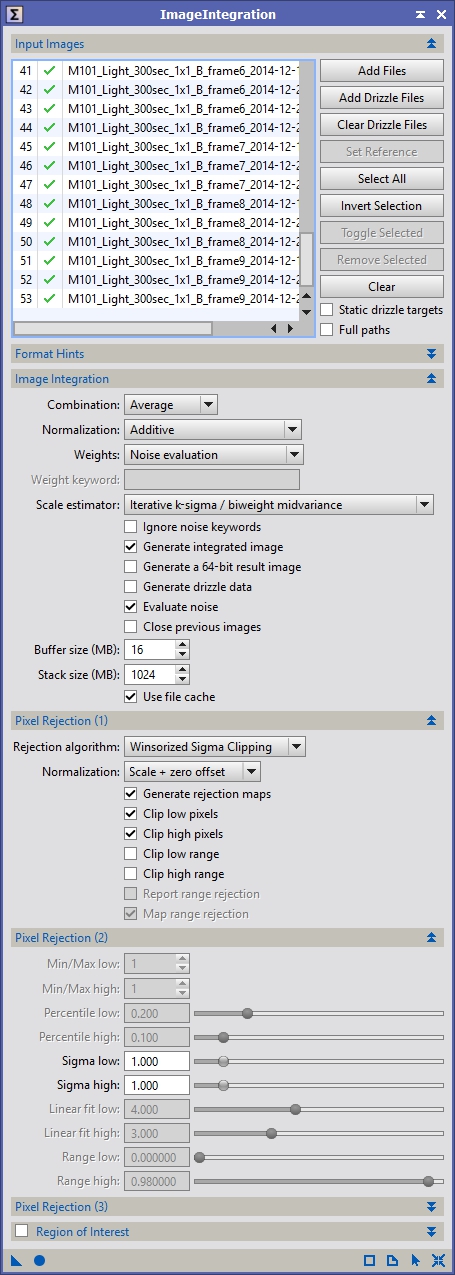
Figure 1: ImageIntegration – Aggressive Rejection
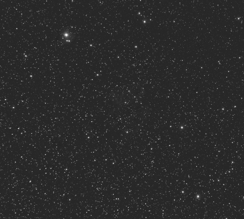
In general, the settings are similar to what I normal default to for light frame stacking, however I set the Sigma low and Sigma high very low so that more stars and nebulosity will be rejected. Figure 2 shows the resulting stack. You can see M101 and a few stars exist but are mostly removed. Hot pixels are still prominent because there was no dithering or calibration to remove them
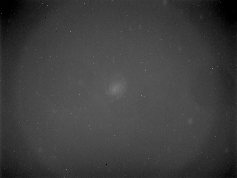
Figure 2: First Pass Synthetic Flat
Let’s get rid of those hot and cold pixels. Bring up PixelMath and put in the following symbols:
f=6.0, w, h, x0, x1, x2, y0, y1, y2, p00, p01, p02, p10, p11, p12, p20, p21, p22, value, sd
And this expression:
w = width($T)-1;
h = height($T)-1;
x1 = x();
y1 = y();
x0 = iif(x1<1, 0, x1-1);
y0 = iif(y1<1, 0, y1-1);
x2 = iif(x1>w, w, x1+1);
y2 = iif(y1>h, h, y1+1);
p00 = pixel($T, x0, y0);
p01 = pixel($T, x0, y1);
p02 = pixel($T, x0, y2);
p10 = pixel($T, x1, y0);
p11 = pixel($T, x1, y1);
p12 = pixel($T, x1, y2);
p20 = pixel($T, x2, y0);
p21 = pixel($T, x2, y1);
p22 = pixel($T, x2, y2);
value = med(p00, p01, p02, p10, p12, p20, p21, p22);
sd = sqrt(bwmv(p00, p01, p02, p10, p12, p20, p21, p22));
iif(p11>(value+(f*sd)), value, iif(p11<(value-(f*sd)), value, p11))
The resulting PixelMath window should look like Figure 3. Apply that to the flat. The resulting image should look like Figure 4. This can also be done with the CosmeticCorrection (CC) tool, but I’ve been using this method since before CC was introduced as a process and I feel I have more control over it this way.
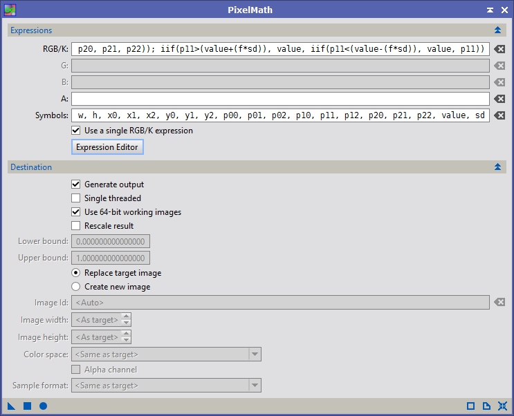
Figure 3: PixelMath – Removing Hot Pixels

Figure 4: Hot Pixels Removed
At this point you could start CloneStamp-ing this image to remove the residual star and galaxy data and depending on size of the structures you are trying to remove with the flat, that might be the correct course. For example, in Anis’ image there is strong vertical banding on the left side of the chip (it’s hidden in the above image due to the vignetting). The scale of those bands are on the order of 30 pixels so to make sure they are corrected by the synthetic flat I can’t do anything to the image that destroys structure sizes over that. Let’s bring up the MultiscaleMedianTransform (MMT) and see if we can improve the image before resorting to the CloneStamp tool.
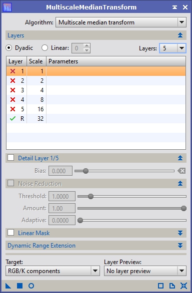
Figure 5: MultiscaleMedianTransform – Removing Small Scale Structure
Figure 5 shows MMT with 5 layers, all 5 of which are disabled. This means that structure sizes from 1 pixel up through 16 will be removed, 32 and above will be retained. When you apply it to the image it will look like the image is blurred but it’s not exactly the same process. I’ve tried this with MultiscaleLinearTransform as well, but I prefer the results from MMT. Figure 6 shows the resulting image.
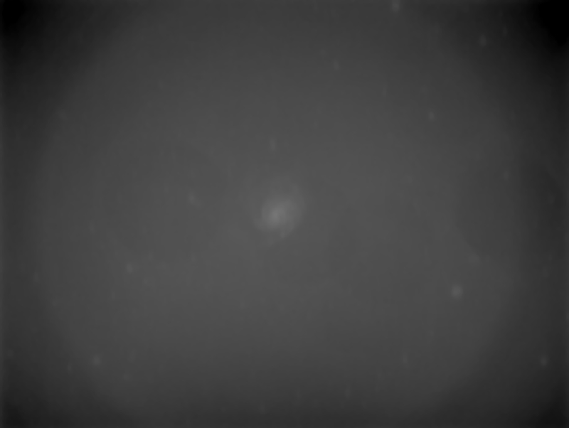
Figure 6: Result of MMT on Synthetic Flat
It’s a little hard to tell from this scaled down image (the original image is 3326 x 25040) but some of the fainter stars and a lot of the small scale noise has been removed.
Next we need to clean up the remaining stars and M101 at the center. Bring up the CloneStamp tool. It is a dynamic process so click on the synthetic flat image window and it will be come the active window. I usually set the opacity very low so that I can accumulate changes. When you are ready to start CTRL click in the image where you want to copy data from and then click on the target you want to replace. Figure 7 shows this process right before I attempt to remove the remnants of the small galaxy to the lower right of M101.
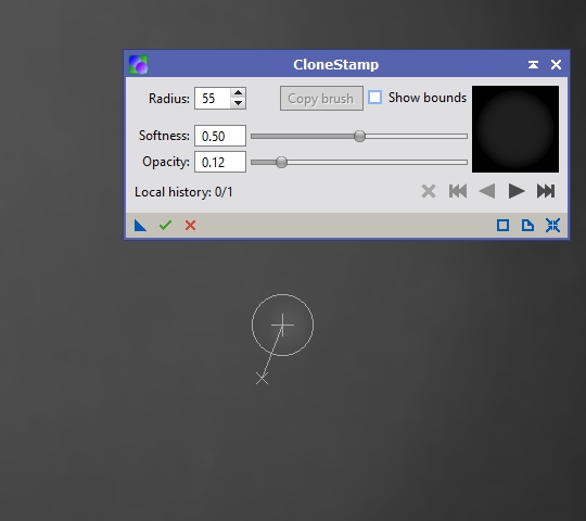
Figure 7: CloneStamp – Removal of Remaining Structures
This is the toughest part of the process. You have to find locations of equal noise and intensity to use as a source for the clone stamp. Vary the size, softness and opacity as you need to remove all the remaining structures. The end result should look something like Figure 8.

Figure 8: Final Flat
You can see that I had to guess at intensity levels where M101 was at. It probably took 50 clone stamp steps to remove all the stars and then another 60 to remove M101. Once you get the hang of it, it goes pretty quickly.
Now that we have a synthetic flat, we need to use it to calibrate our images. I started with uncalibrated data so this synthetic flat needs to be applied to the uncalibrated subs. If you have darks, bias or flats, you should run 2 calibration steps. First calibrate with the normal calibration frames then run through this process using the calibrated subs to create the synthetic flat then calibrate the calibrated subs with the new flat (darks and bias disabled). Figure 9 shows how I typically run ImageCalibration with the synthetic flat.
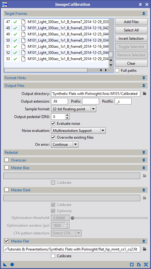
Figure 9: ImageCalibration – Using Synthetic Flat
We should now have a set of well corrected sub frames that we can stack. Go through your normal process to register and integrate these. You can use my PixInsight Manual Image Calibration, Registration and Integration tutorial if you need more details on those processes.
Figures 10 through 13 show a comparison of the synthetic flat vs no correction, ABE & ABE+DBE.

Figure 10: No Correction
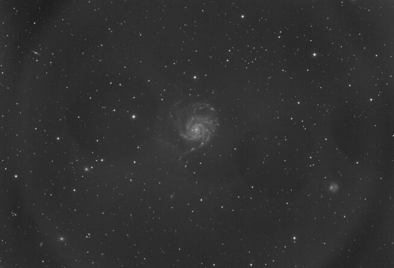
Figure 11: ABE only
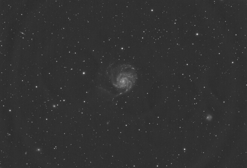
Figure 12: ABE + DBE
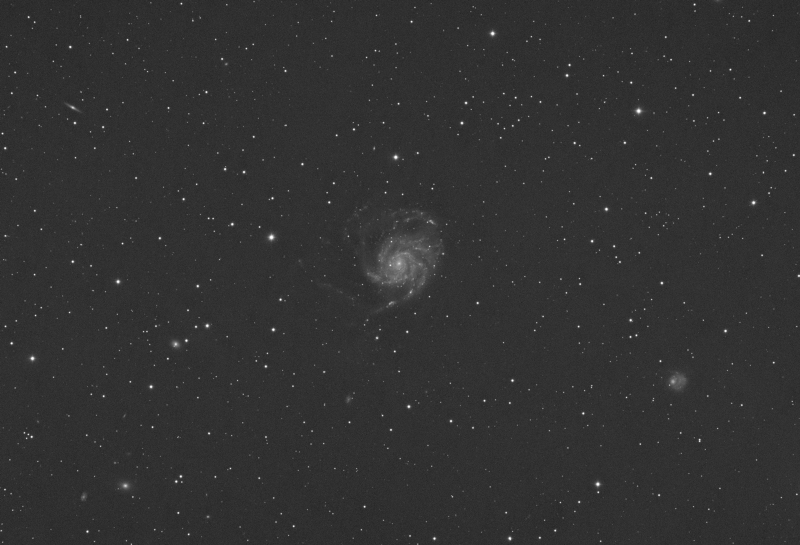
Figure 13: Synthetic Flat Correction
While the synthetic flat is not perfect it can do a much better job than ABE or DBE in many situations.
Synthetic Flat Creation from a Single Image
If you are starting with a single frame then, like I said, the process is very similar. You run MMT to remove most of the structures, although if you have vertical or horizontal banding in your image like Anis has then instead of MMT try using the Superbias process. It uses a MultiscaleMedianTransform process but only in one direction so it will protect the direction opposite of the one it is blending. For example, if you set it to Columns it will run MMT vertically, but not horizontally. If I start with Figure 10 as the main image then to create a synthetic flat for it I would use Superbias as shown in Figure 14.
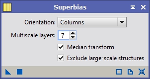
Figure 14: Superbias – Used for Synthetic Mask Creation
Figure 15 shows the initial synthetic flat created by running Superbias on the image from Figure 10. Figure 16 shows the Synthetic flat after some CloneStamp work. Figure 17 shows the calibrated version of Figure 10 using the synthetic flat from Figure 16.

Figure 15: Synthetic Flat from Superbias

Figure 16: Synthetic Flat after CloneStamp
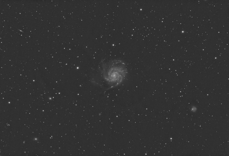
Figure 17: Image After Synthetic Flat Correction
One other tip. You can combine ABE, DBE and synthetic flats to get better results. For example, you could remove M101 by running DBE on the synthetic flat before starting the CloneStamp work then use the background created by DBE (resized to the original image) as the source for CloneStamp to remove M101 (see Figure 18). The reason I didn’t do this here is there is a dust shadow that M101 straddles in this image and I wanted to keep that intact if possible.
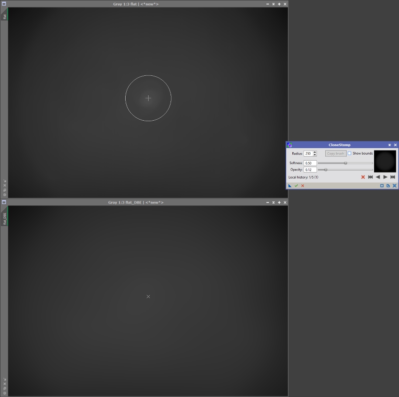
Figure 18: CloneStamp from DBE of SyntheticFlat to Remove Structures
I hope everyone finds this useful and if you have any questions about this tutorial please let me know.
Interesting stuff!
Do you have any tip how to use this technique to get rid of reflections. It is hard to remove nebulosity with clone stamp. So I wonder if there is Pixel Math formula to subtract the artifacts
Reflections look like this
http://www.astrobin.com/224948/
Mark
Hi Mark,
Those are very tricky. I wouldn’t say it’s impossible, but you really need to know what structures are real and what isn’t. I took a quick stab at your data and came up with this:
Resized to 800×718 it looks great, but at full size there are many artifacts around the reflection areas. I also wasn’t sure if there was any nebulosity in the area so it’s possible I removed things that shouldn’t have been or left things in that should have been taken out.
To do this, I cloned the image then did a star removal (see my tutorial other tutorial on that. Then I used the MultiscaleMedianTransform with the first 3 layers disabled to remove any other star remnants. There was a lot of clone stamping involved to remove any stragglers. Instead of applying it as a flat (division) I subtracted it. I called the modified image ‘background’ and then ran this PixelMath expression on the original image: $T – background + med(background)
If you spend a lot of time on this you could probably get it all cleaned up with little loss of data even at full resolution.
Regards,
David
Thanks David!
Was very useful. Looks I have tonnes of these rings popping out from all corners. I feel I will get back on this.
Cheers
Mark
The best solution is obviously to kill the internal reflections at their source but that isn’t always possible. Are you using an SCT with a F/6.3 reducer? That combination is notorious for problems like this. I’ve seen lots of potential fixes, like using a black marker on the outside of the reducer lenses but I have no idea how effective they really are.
Regards,
David
Very helpful! I saw your post on the PI forum. At what point during this process would you employ your strategy for removing the donuts or would you ignore the donuts until the image is non-linear, then deal with them?
Thanks
Dave
Hey Dave,
Depending on the size of the donut using a synthetic flat should should remove the donut as well. I got the idea for the synthetic flat from observatories which frequently use night time sky flats where they take normal images moving the scope to different locations and then stack them without registration. The rejection methods remove all stars and spurious data leaving them with a very good ‘flat’. Most of the space based observatories have no choice but to use this method. A synthetic flat is similar in that you are using real light data to generate the flat, however stars, galaxies and nebulosity may still be present and need to be removed first for it to work. Shadows, vignetting banding, etc. should all still be present in the image after this process so they should be removed from the image after calibration.
Regards,
David
Ok great. Thanks again! I’m going to give this a try and will let you know for sure if it works. So far nothing else has!
Dave
Hi Dave,
I’ve used your PixelMath for removing hot pixels from subs where dark, flat and bias frames don’t seem to touch them (an old Canon 350D as the source and guided exposures of 10 minutes). It works surprisingly well, although I find I have to run it between 5 and 10 times to remove all of the hot pixels. This is on a calibrated, registered and debayered sub.
I suppose my questions are:
1. Would you recommend this only for use on debayered subs?
2. Is there a way to tune the hot pixel removal from the PixelMath expression? The “f=9.0” looks like the place I could try perhaps?
3. Is there a way of running this multiple times automatically do you think?
Thanks in advance for any thoughts.
Phil
Hi Phil,
Let’s see if I can answer all your questions:
1) Yes, the subs would need to be debayered first. This is because, while Bayered, the intensity at each adjacent pixel may be very different due to the filter transmission and brightness of the object in each portion of the spectrum that the filter allows through (this is why with Bayered data you may see some pixels as much darker than others when zoomed in). The expression could be modified to work on a Bayered image but it would be difficult and easier to do with a script or process.
2) Yep, the f=9.0 is essential a sigma multiplication factor. It isn’t exactly a sigma value because I’m using a biweight midvariance function instead of standard deviation, but it works effectively the same way. Smaller values will mark more pixels as hot or cold and replace them with surrounding data, so they are more aggressive but they also have a higher chance or removing real data, like star peaks.
3) If you bring up the ProcessContainer you can drag the ‘new instance’ icon from the PixelMath window into it 5 or more times. When that ProcessContainer is applied to your image it will run that PixelMath expression however many times you added it in. You can save that ProcessContainer off, just like the PixelMath process so it can be used whenever you want.
I will say that when I created some of these PixelMath expressions, tools like CosmeticCorrection did not exist. The ‘Use Auto detect’ option does essentially this same thing. It does use standard deviation rather than bwmv which is not as robust but still works well. It also only works in a global capacity on files, so you can’t run it on a single image or use the ProcessContainer method I described above to run it in multiple passes. It does however handle Bayered data (the CFA option – which stands for color filter array).
Let me know if I didn’t answer your questions fully or you had any others.
Regards,
David
Your pixelmath statement is not longer valid. It contains errors.
I tried it straight as you have it and then modified it to try and get it to work to no avail.
Process console below:
PixelMath: Processing view: integration1
Writing swap files…
117.023 MiB/s
*** Error: Invalid character in expression:
w = width($T)-1;
h = height($T)-1;
x1 = x();
y1 = y();
x0 = iif(x1<1, 0, x1 – 1);
y0 = iif(y1w, w, x1+1);
y2 = iif(y1>h, h, y1+1);
p00 = pixel($T, x0, y0);
p01 = pixel($T, x0, y1);
p02 = pixel($T, x0, y2);
p10 = pixel($T, x1, y0);
p11 = pixel($T, x1, y1);
p12 = pixel($T, x1, y2);
p20 = pixel($T, x2, y0);
p21 = pixel($T, x2, y1);
p22 = pixel($T, x2, y2);
value = med(p00, p01, p02, p10, p12, p20, p21, p22);
sd = sqrt(bwmv(p00, p01, p02, p10, p12, p20, p21, p22));
iif(p11>(value+(f*sd)), value, iif(p11<(value-(f*sd)), value, p11))
…………….^
Reading swap files…
1455.921 MiB/s
PixelMath: Processing view: integration1
Writing swap files…
120.349 MiB/s
*** Error: Invalid character in expression:
f=6.0; w = width($T)-1; h = height($T)-1; x1 = x(); y1 = y(); x0 = iif(x1<1, 0, x1 – 1); y0 = iif(y1w, w, x1+1); y2 = iif(y1>h, h, y1+1); p00 = pixel($T, x0, y0); p01 = pixel($T, x0, y1); p02 = pixel($T, x0, y2); p10 = pixel($T, x1, y0); p11 = pixel($T, x1, y1); p12 = pixel($T, x1, y2); p20 = pixel($T, x2, y0); p21 = pixel($T, x2, y1); p22 = pixel($T, x2, y2); value = med(p00, p01, p02, p10, p12, p20, p21, p22); sd = sqrt(bwmv(p00, p01, p02, p10, p12, p20, p21, p22)); iif(p11>(value+(f*sd)), value, iif(p11<(value-(f*sd)), value, p11))
………………………………………………………………………..^
Reading swap files…
1476.639 MiB/s
Hi Aaron,
I’m not sure exactly what happened but something is wrong with that expression. I believe on the 5th line there is a ‘dash’ character rather than a minus sign. Also, the y0 expression looks incorrect and the x2 expression is missing. Just in case, I’ve uploaded a desktop icon with the correct expression here. Download that zip file, extract it and you should be open it with PixInsight either by dragging the file over or by right clicking on the PI desktop and going to Process Icons->Merge Process Icons… and select the xpsm file. It should show up on workspace01 in the upper left corner.
Regards,
David
That makes sense. Perhaps some font misinterpretation from my browser to PI.
Thanks for the sharp eye!
Now that Local Normalization (and Large Scale Rejection) are available- do you think they can be used in lieu of the process above? I hope so… However, I cannot seem to get LN to do the job on a set of data that has most good calibrated frames- with a handful of data that do not have flats (but otherwise the data is good).
Hi Adam,
We’ve talked on the side, so I’m approving your comment. Sorry for the slow response.
Regards,
David