Overview

PixInsight has some fantastic tools and there are some nice wrappers around them, like the BatchPreprocessing script, that make them easier to use and and more efficient.  The problem with simplifying is that you also loose access to detailed controls and many of the operations of the base tools are hidden.  I’ve found that by using the individual tools I can get a better result and increase my understanding of what is actually happening at each step.  For these reasons, I put together this tutorial on how to manually calibrated and stack your data using PixInsight.

I’ve broken this tutorial down into a few categories.  Image calibration (also called reduction) is the process of using calibration frames to help remove fixed patterns from your data to improve the accuracy of the signal acquired in your light frames.  Calibration frames come in several categories: bias, dark & flat.  Each one is acquired and utilized differently.  Registration is the process of aligning the images.  Integration (also called stacking) is the combination of individual frames to create a single image, typically with a view of increasing the signal to noise ratio (SNR).

Update 2015/11/20

The text in the section about image integration is correct, however the image did not match.  The normalization mode was set to ‘Additive’ when it should have been ‘Additive with scaling’.  I’ve updated the figure to reflect that.

Update 2015/07/02

I should make it clear that the first part of this tutorial covering master calibration frames and image calibration can be done reasonably well by the BatchPreprocessing (BPP) script for 90% of the data sets we have.  However, BPP has it’s limitations (only one set of darks is allowed, limited control of integration settings, etc.) and when problems occur it is good to understand what it is doing under the covers so you can debug or step away from BPP if it is limiting you.

Update 2015/05/15

I did a presentation on the Astro Imaging Channel that covered this same material (plus a couple bonus  items).  You can find the Youtube video of it here.

Image Calibration

NOTE: If you are using a DSLR or OSC CCD I would suggest not Debayering your data until after calibrating.  OSC CCD data has to be Debayered manually any way, but by default PixInsight Debayers DSLR raw data.  This can be disabled by going to the Format Explorer tab and double clicking the DSLR_RAW format.  Select the ‘Create raw Bayer CFA image’ option.  Alternatively, the latest updates to PixInsight add a new button to this form called ‘Pure Raw’ which sets everything up so the image is interpreted exactly as it is stored in the raw file.

Bias Frames

Bias frames are trying to capture the fixed pattern that occurs when reading your sensor.  Since it takes time to read out the data from a standard CCD camera thermal and electronic noise can build up in different ways depending on when a particular pixel was read.  This creates a repeatable pattern that can be removed with bias frames.  There is also random noise that goes along with this pattern called read noise (or read-out noise).  This noise cannot be removed but it can be reduced and in order to get the best picture of what the bias pattern looks like we need to reduce the random portion as much as possible.  We do this by stacking multiple frames.  Stacking, or averaging data from multiple frames, increases the signal linearly but because the random noise follows a Gaussian distribution it only increases as a square root function, so the more of them we combine the more we can separate the signal from the noise.  For example, if we take the value of the same pixel over multiple frames we may get a sequence like this:

240, 267, 215, 225, 205, 280, 211, 190, 241, 203

If we just took one frame we would have a value of 240 for that pixel, but you can see that over time the intensity varies due to the random noise.  If we average them we get a value of 227.7 which will be much closer to the real signal value.  The more data points we average the closer we get to the true value.

To take bias frames make sure that the shutter is closed and/or the optics are sealed so that no light is reaching the CCD and then take the shortest exposures possible.  Take as many of these as seems reasonable.  Here’s why:

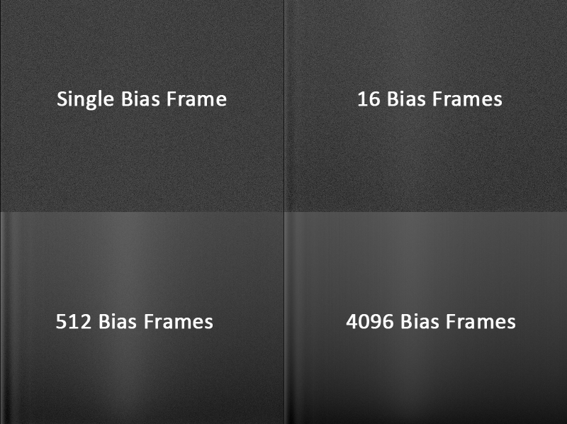
Figure 1: The effects of stacking bias frames

You can see in Figure 1 that using just a single bias frame give you just a bunch of noise.  Stacking 16 gives you a much clearer picture of what the fixed bias pattern looks like.  By the time we get to 512 or even 4096 bias frames the bias signal is very clear and most of the noise is gone.

Taking 4096 bias frames isn’t the most practical solution though.  Enter the SuperBias process.  Since most bias frames are strongly column or row oriented you can remove a significant amount of the high frequency noise with this tool while keeping the real bias signal.

Figure 2: Super bias vs. hard work

I still recommend taking and stacking around 25 to 50 bias frames before running SuperBias but it can really clean up your master bias frame.  To stack your bias frames bring up the ImageIntegration process and load your bias frames by clicking on the ‘Add Files’ button.  These are the settings I use:

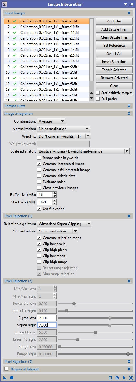
Figure 3: Integrating bias frames

We want a straight average of this data with only a minimal amount of sigma rejection to catch cosmic ray strikes.  Sigma rejection uses standard deviation to determine outliers.  To understand this, let’s take the same set of values we used before for the same pixel in different bias frames:

240, 267, 215, 225, 205, 280, 211, 190, 241, 203

Here the average is 227.7 but you can see that some values are quite far away from that average.  The standard deviation gives us a way to measure the variation in the set of pixel values and we can use it to identify outliers.  In this case the standard deviation is 29.1 (one standard deviation is called sigma or σ).  If we rejected pixels that had values outside of 1σ then we would throw out the values of: 267, 280 and 190.  A pixel with the value of 402.3 would have a value of 6σ relative to the set listed above.  Of course as you get outliers this shifts the average and standard deviation.  This is another reason for taking lots of frames.  The more data you have in your set the easier it will be to identify outliers from the rest of the set.

I usually use values of 6 to 10 for the sigma rejection depending on how noisy the data is.  If you want to understand more of the math involved and all the details about image integration you should look into PixInsight’s own documentation on this.  It gives you more information than you will likely every want to know unless you are a total math junkie.

 

Dark Frames

The next calibration frame type is darks.  A dark frame is designed to capture the fixed pattern that builds up over the duration of a normal light exposure due to thermal and electrical influences.  This can take the form of hot and cold pixels as well as thermal variations across the chip due to adjacent circuitry and the sensor itself.  Darks are taken similar to bias frames: the OTA or camera system should be sealed so that no light reaches the sensor and then take exposures equivalent to your light exposure lengths.  For example, from my backyard I can rarely expose for more than 5 minutes while using wideband filters like LRGB, so I would take 5 minute darks to match the exposure of my lights.  In addition to matching exposure time you also need to match temperature.  How the dark noise accumulates over time is highly temperature dependent.  The KAF based cameras (KAF 8300, 16803, etc.) tend to have doubling temperatures of around 6°C.  This means that if the temperature of the sensor increases by 6°C the dark noise is doubled.  This is the main reason for cooling imaging sensors.  Most modern CCD cameras have thermal regulation making temperature matching much easier.

When creating the master dark I use essentially the same ImageIntegration settings as I did for the master bias (see Figure 3).  Again, I may alter the sigma rejection parameters based on the noise and number of dark frames I have.

 

Flat Frames

The next calibration type is flat frames.  These capture all of the variations of how light is accumulated by the sensor including how the light moves through the optical system and how sensitive of pixels vary across the chip due to the manufacturing process.  The most obvious of artifacts captured by flats is vignetting and dust shadows.  Unlike the other two calibration frame types, flats need to be taken with light falling on the sensor and in order to take a picture of all the variations we need to take a picture of the most even light source possible.  Many people use flat frame devices like flat boxes and electroluminescent panels and others use sky flats, usually with some sort of diffuser (i.e. a white t-shirt or sheet of paper) over the optics to further even out the light variations.  Either method works, but the advantage of the flat frame devices is that their light output is generally consistent enough that you can always use the same exposure times.  You also don’t have to worry about taking flats at a specific time (usually dusk or dawn).

To take flat frames point your scope at the zenith or your flat frame device and take an exposure so that the average ADU (analog to digital unit) is around ¹/₃^rd to ½ of the maximum value (for a 16 bit sensor the max is 2^16 = 65535 giving a range of around 20k to 30k).  This range is usually safe but really all you need is for the normal distribution of the image data to be far enough away from the minimum and maximum values so that no pixels values are clipped and for the data to all be within the linear range of your sensor (I’ll cover CCD characterization in a different post).  You’ll want to take flats for each filter (assuming you are using filters) and for every orientation of the camera relative to the optical system.  This is because each filter will have different responses to the light passing through them.  They might have dust in different locations causing different shadows.  Also, the vignetting will change relative to the camera if it is placed in a different orientation relative to the optics.  Like the other calibration frames, you’ll want several flats to minimize the noise in your master flat frame.  I usually target at least 25 per filter.

Once you have your flat frames we need to calibrate them.  The flat image contains the bias data as well dark current noise and this creates an offset that needs to be removed before we can calibrated the light frames with the flats.  If your flat frame exposures are very short, which is generally the case, you can get typically just use the master bias to calibrate the flats.  If you have long exposure flats and a high dark current camera you may want to take dark flat frames and create a master dark flat.  These are just like dark frames except taken at the same exposure length of your flats.

If you are using bias frames to calibrate your flats I use ImageCalibration with the settings in Figure 4.  Figure 5 shows the settings for calibrating with dark flats.

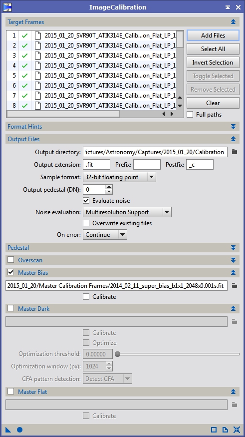
Figure 4: Flat calibration with master bias

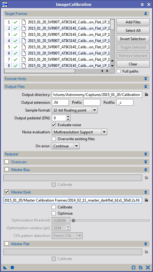
Figure 5: Flat calibration with master dark flat

We should now have a bunch of calibrated flat frames that we need to combine into a master flat.  Bring the ImageIntegration tool back up and select all your calibrated flat frames.  We are going to use very different settings from what we used for the dark and bias master frames.  First, in the Image Integration section we are going to use Multiplicative normalization.  This is designed specifically for images that will be used to multiply or divide another image later on, which is exactly what we do with the master flat when calibrating light frames.  In the Pixel Rejection (1) section again, we change the Normalization setting to Equalize fluxes.  This just increases or decreases the total energy so that the peak of the histograms match between subframes.  This works better for sky flats which might have highly variant energy levels between the first and last frame.  If you are using a light box or electroluminescent panel you can probably use one of the other methods, but I generally just leave this on Equalize fluxes when integrating flats.  I also allow a little more aggressive sigma rejection settings with flats.  Figure 6 shows the settings I typically use.  Figure 7 shows a typical master flat stretched so we can see the artifacts we are trying to correct with it.

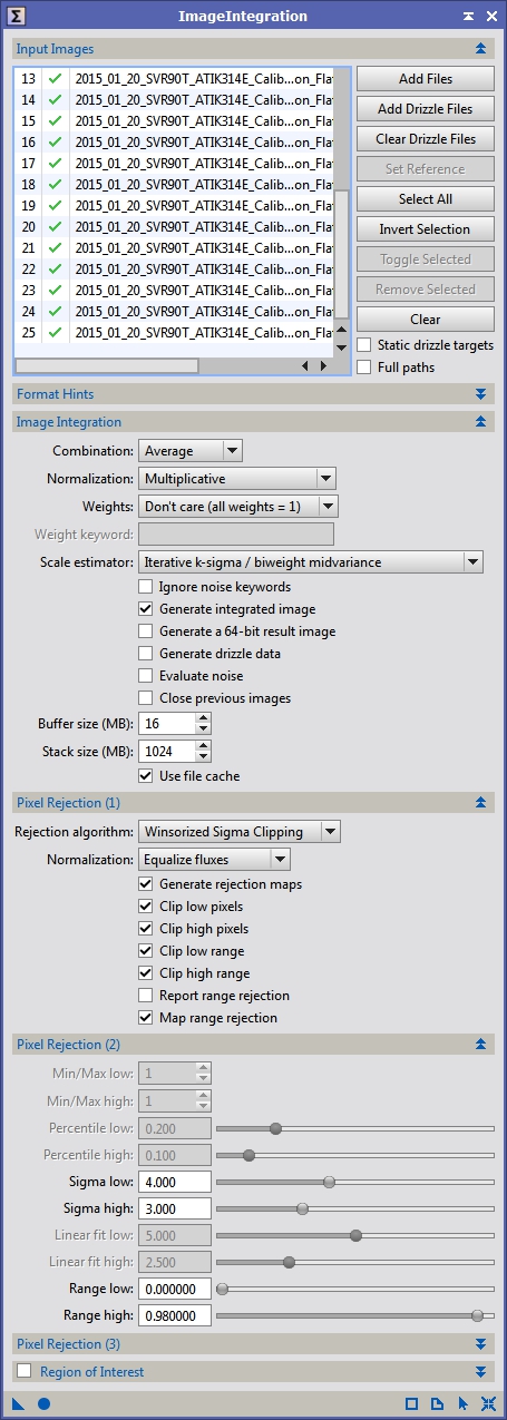
Figure 6: Integrating flat frames

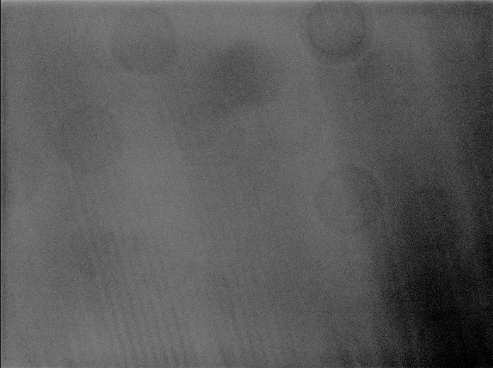
Figure 7: Master flat (stretched for visibility)

 

Light Frames

We should now have all the data we need to calibrate our light frames.  Bring up the ImageCalibration tool again and select all your light frames.  If you are using a filter wheel and have data with different filters make sure to calibrate them separately with the appropriate master flat (and master dark if you are using them and they are of different exposure lengths).  There are multiple ways to handle the calibration of light frames mostly dealing with what each master frame was calibrated with.  Did you bias subtract your darks before integrating them?  Did you just average your flats without bias or dark subtracting them?  Are you going to scale your darks?  In general, I prefer to not bias subtract my darks because the dark current in my sensor is very low and this can lead to underflow issues; meaning any given pixel in my bias frame could have a higher value than the corresponding pixel in my dark frame so when I subtract them I would get a negative value.  Since most programs clip negative data this leads to incorrect information in the calibrated and master darks.  This isn’t a problem with flats and lights since the background level is generally well above the bias level (this isn’t always the case especially if you are doing narrow band imaging so you still have to be careful).  The following figures show the settings I use for different scenarios.

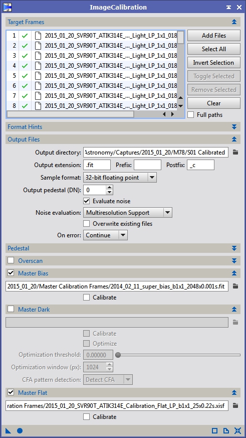
Figure 8: Light frame calibration using a master bias and a bias subtracted master flat

 

Figure 9: Light frame calibration using a master dark and a bias or dark flat subtracted master flat

 

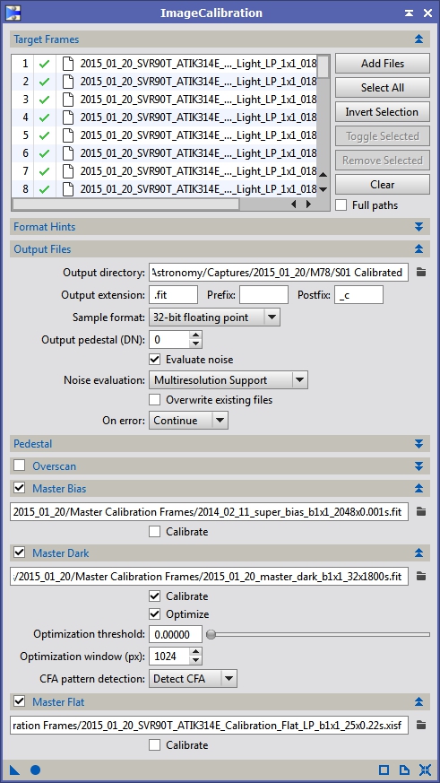
Figure 10: Light frame calibration using a master bias, master dark with scaling enabled and bias or dark flat subtracted master flat

 

Bad Pixel Maps

At this point you should have a set of calibrated light frames, however before we move on to registration and stacking I want to talk about another method to remove hot and cold pixels.  You might consider this if you are not using a thermally regulated camera especially if you don’t even have a temperature read-out on the sensor, like my ATIK 314e.  This process is called a bad pixel map or sometimes a defect map.  The idea is that you identify the hot and cold pixels and create a map of them.  Then you run a process that replaces each hot/cold pixel with the median value from the surrounding pixels.  Some processes allow you to replace the defective pixel with a Gaussian sampling, box average, minimum, maximum, etc. of surrounding pixels.  Whatever the specific algorithm the bad pixel is replaced with a value that is likely to be more accurate.  Because my camera has very low dark current, few hot/cold pixels and is not thermally regulated this is the process I use when calibrating my images.

Generally the bad pixel map is created from a master dark, but it can be created manually or by rejection algorithms as well.  PixInsight has two tools for applying a bad pixel map, the first is fairly straight forward.  If you have a defect map already, you open it up, select the defect map view and apply it to your image (or use it in conjunction with an ImageContainer to apply it to all of your images).

Figure 11: DefectMap Tool

If you have a master dark or want to use rejection to detect the hot pixels you can use the CosmeticCorrection tool.  I do like the control that DM gives you for how a pixel is replaced, but given that there is no longer an automated tool for creating a defect map I think using CC is probably the way to go for most people.  Figures 12 through 14 show the different ways of using CC to fix bad pixels.  The first method uses a master dark frame to identify hot and cold pixels.  When run, CC will replace all pixels identified in each of the calibrated sub frames with data from the surrounding pixels.  I’m not sure what algorithm CC uses under the covers but my guess is a median function.  The second method looks at a small window of pixels and identifies any pixels that are beyond the sigma levels defined and then replaces them.  This works well for stuck pixels that are 100% on or off but because there aren’t that many pixels in the pixel window for analysis I’ve had trouble with it either not detecting hot/cold pixels or unintentionally replacing the peaks of small stars.  The last option is entirely manual.  You enter what row/column your bad pixels are in or if you have an entirely bad row/column and it will then replace those pixels with better data.  One other thing to note, if you are using a DSLR or OSC and are processing your data as RAW at this point (which is what I suggest) you should turn the CFA option on.  This makes it so the hot pixel identification and replacement algorithms work correctly with Bayer matrix data.

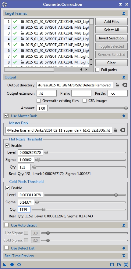
Figure 12: CosmeticCorrection using dark frame to identify hot/cold pixels

 

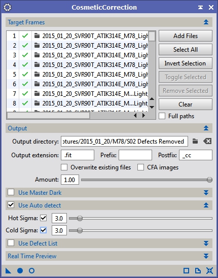
Figure 13: CosmeticCorrection using standard deviation to detect single pixel outliers and replace them

 

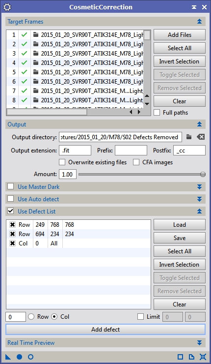
Figure 14: CosmeticCorrection using a list of defects

 

Image Selection and Weighting

NOTE: If you are imaging with a DSLR or OSC CCD I would suggest Debayering your images at this point.  They don’t necessarily need to be Debayered for SubframeSelector, but the Bayer matrix intensity differences can sometimes cause problems when measuring stars.  You definitely need to Debayer your data before registering it though.

Now that we have calibrated and cleaned up data we could immediately jump to registration (aligning the images).  However, there’s another tool in the PixInsight arsenal called SubframeSelector that can greatly enhance your results if we use it before registering our data (it can be thrown off by using registered data which might have regions with no information).  The original point of SubframeSelector was simply to identify light frames that might have issues that were severe enough you might not want to include them in your final stack.  This could be from a cloud passing through the field of view, a piece of grit sticking in your gears and throwing off your tracking, focus slipping, etc.  It also supports the ability to add a keyword into the FITs header that can be used by ImageIntegration later on to weight how the images are combined.  This is exceptionally useful if you have data from multiple sessions or instruments where the SNR or resolution my vary considerably.  By weighting images you can control how much influence an sub frame with a lower SNR has on the final integrated image.

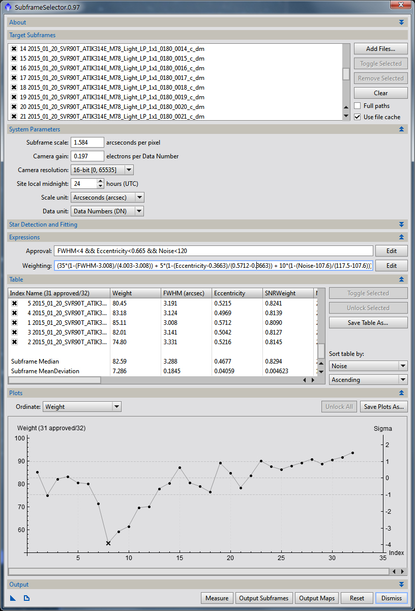
Figure 15: SubframeSelector

SubframeSelector’s use is fairly straight forward.  You give it a list of images (Figure 15, Target Subframes), put in some information about your camera (Figure 15, System Parameters), tell it what restrictions you want to use for approving images and how you want to weight the combination of that data with ImageIntegration (Figure 15, Expressions) and then measure and output your approved frames.  As you can see from Figure 15, I’ve am limiting the approved images to frames that have a FWHM less than 4 arc-seconds.  FWHM is the full with at half maximum of a point spread function (PSF) and in astronomy since stars are true point sources their FWHM can be used to understand what is actually resolveable in the image.  Smaller FWHM values are better.  I’ve also restricted the list by the Eccentricity and Noise metrics.  Noise is fairly straight forward, the higher the noise level the more difficult it is to discern your target, so again, lower values are better.  Eccentricity is a measure of how far from round a star is.  If a star is very elongated it will have a higher Eccentricity value, so it is also better to have lower values here.

The weighting is more complicated.  Here is the full equation I used in Figure 15:
(35*(1-(FWHM-3.008)/(4.003-3.008)) + 5*(1-(Eccentricity-0.3663)/(0.5712-0.3663)) + 10*(1-(Noise-107.6)/(117.5-107.6)))+50

It looks like a bit of a mess, but if we break it down it’s not difficult to understand.  The first term is: (FWHM-3.008)/(4.003-3.008).  Really all I’m doing is normalizing the FWHM values to a range of 0 to 1.  I subtract the FWHM for a given image by the minimum value and the divide by the range of values.  So, when FHWM is the maximum value I get (4.003-3.008)/(4.003-3.008) or 1.0.  You can see I do this for all the terms I’m interested in.  Unfortunately, SubframeSelector doesn’t currently have a FWHMmax or FWHMmin variable so you have to sort the list and manually enter the min/max values for each term.  The next thing I do is invert those terms, which is where the 1-x comes from.  This simply takes each term which are now ranging from 0 to 1 and makes them range from 1 to 0.  This way if I have a large FWHM image it will have a lower weighting value, since larger FWHM values are worse.  If I was using the SNRWeighting term I wouldn’t include a 1-x term since larger values are  better.  Next I weight each term by its importance to me.  For example, I’m more interested in getting the highest resolution possible so I increase the FWHM terms resulting value relative to the other terms.  This is what the 35, 5 & 10 values are for.  If you were less concerned with resolution and wanted rounder stars with a better SNR then you might weight FWHM lower and Eccentricity and Noise higher.  I’ve chosen the weighting values so that my result will be in the range of 0 to 50 and then I add 50 to the entire expression so that the final range is 50 to 100.  I could have used a 0 to 5 or 0.5 range and it wouldn’t really matter, but the offset is important.  By forcing the weighting range to be 50 to 100 I make sure that even the worst frame still has a reasonable contribution to the final ImageIntegration result since its weight is never less than half the maximum value.  If I left the range as 0 to 50 then the worst frame would not contribute to the final image at all.

Now that we’ve approved and weighted our images, we want to annotate them with that information and output them so we can use them for registration and integration.  In the output panel (see figure 16) select the directory where you want your images to go, how you want them tagged and define what the Weight keyword will be (I chose SFSWEIGHT for Sub Frame Selector Weight).  We will use the weight keyword later on in ImageIntegration.  Click the Output Subframes button and you’ll now have a directory full of calibrated, defect corrected and weighted light frames.

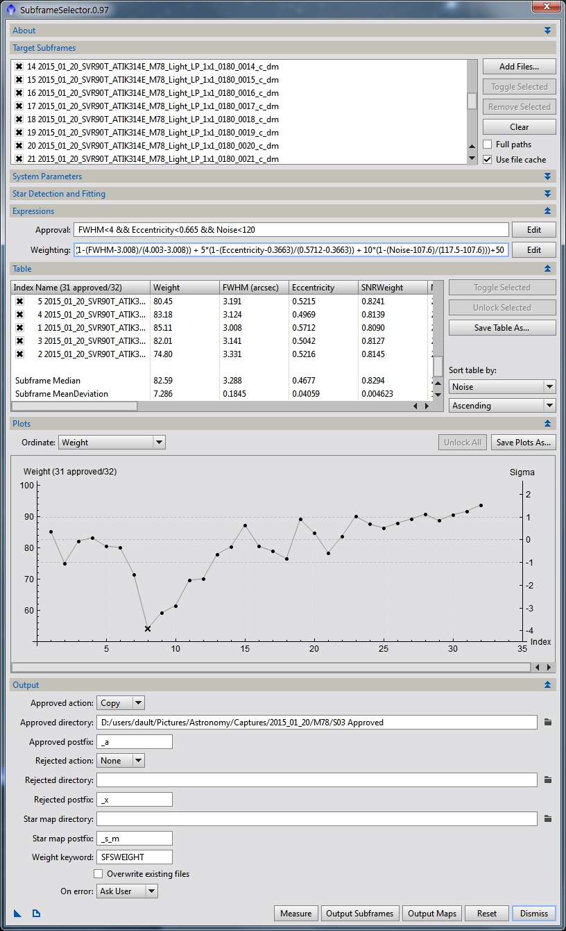
Figure 16: SubframeSelector with Output panel shown

 

Registration

Next on to registration.  Bring up the StarAlignment tool (see Figure 16) and select one of your approved images that best represents the field of view you want from your final stack.  Honestly, I typically just use the first image in the list since when I captured the data that’s what I framed, picking which frame is the reference will be more important when we get to ImageIntegration.  I typically use the Distortion correction option.  This is designed to correct minor deviations of star positions due to scintillation effects, tracking elongation, etc.  On rare occasions I’ve noticed a little color separation between a color filter image and my luminance data on some stars that was fixed when Distortion correction was enabled.  Theoretically, it could improve the star sizes as well since the stars should overlap more precisely but I have not measured a difference.  I keep it on since it generally adds very little processing time and meets the distortion residual in just a couple iterations rather than the 250 I set.

For most registration purposes we use the Register/Match Images working mode.  I’ve only ever deviated from this if doing mosaics.  Next select all your approved images with the Add Files button and set the output directory for your registered data.  For the most part, you probably won’t have to alter the Star Detection or Star Matching parameters.  If you have a really large (or small) image scale or are combining data from imaging systems with different image scales then you may need to make changes here, but otherwise I leave these alone.  I prefer the Lanczos-5 interpolation method.  It seems to do a better job of dealing with small rotational and scale differences than some of the other methods.  I do sometimes get ringing around stars and will have to alter the clamping threshold or choose a different method.  I generally test registration on a single frame first to see if there are any artifacts like this before running it on all images.  Once you are set, hit the Apply Global button (the little filled circle at the bottom left) and wait.

NOTE: You can register all your data regardless of filter or instrument to the same reference frame.

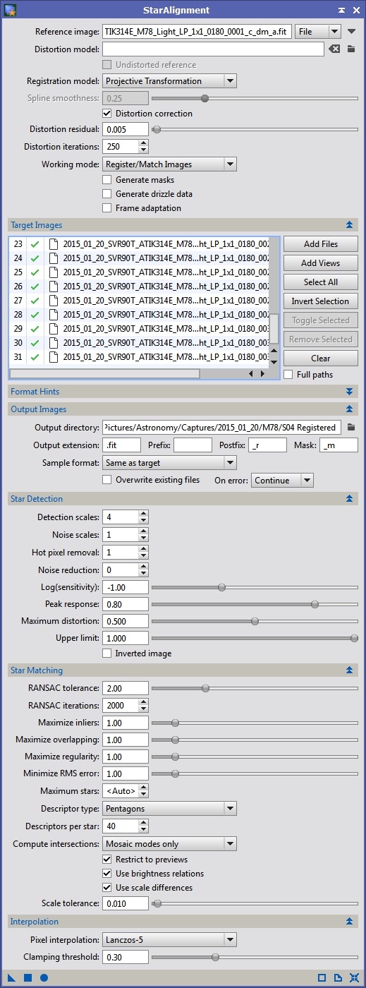
Figure 17: My StarAlignment typical settings

On rare occasions some images are not registered.  Usually this is because I’m trying to include an image that has severe tracking issue or I’m combining data from different instruments with different orientations and image scales.  The number of successfully registered images should be reported in the console along with the number of failed alignments.  The common thing I have to change when working with data of different scales is the Detection scales setting.

 

Image Integration (Stacking)

Now we should have calibrated, defect corrected, approved, weighted and registered data and it’s time to stack them.  Unlike registration we want to stack data from different filters separately (although you can certainly combine data from different instruments provided the light is passing through similar filters).  Bring up the ImageIntegration process (see Figure 18) and select your registered data.  We want to be careful about which frame is used as the reference.  Pick your best frame by using the highest weighted image from SubframeSelector or manually examine all frames with the Blink tool.  Ideally your reference frame shouldn’t have satellite trails and should be free of gradients as well.  Select that image from your target frame list and click the Set Reference button.

For light frames we want to use an Average combination with an ‘Additive with scaling’ normalization (used when summing or averaging data which is what we are going to do).  Pay special attention to the Weights method.  You can see in Figure 18 I’ve selected FITS keyword and specified the Weight keyword of SFSWEIGHT which is what we defined using SubframeSelector.  By default, ImageIntegration sets the Weights to Noise evaluation which weights the image combination by their noise values.  By specifying the SubframeSelector weight keyword we can alter this to target specific features, like maximizing resolution over SNR.  Most of the other settings in the Image Integration panel I leave alone.  I typically use Winsorized Sigma Clipping with a Scale + zero offset normalization for the pixel rejection.  I’ve found this method to give the best rejection of true outliers with few incorrectly rejected pixels (by incorrect I mean data that I would want included not that the algorithm is faulty).  I generally use a sigma of 4.0 for low value rejection and 3.0 for high value rejection.  Spurious low values tend to be just random noise but high values tend to come from cosmic ray strikes, hot pixels not caught by the previous steps and random noise.  This is why I’m more restrictive with the high range sigma.  Once you have set all your options hit the Apply Global button and wait.  If you have the Generate rejection maps option checked you should get more than just your integrated frame, you’ll also get frames showing you what pixels were rejected.

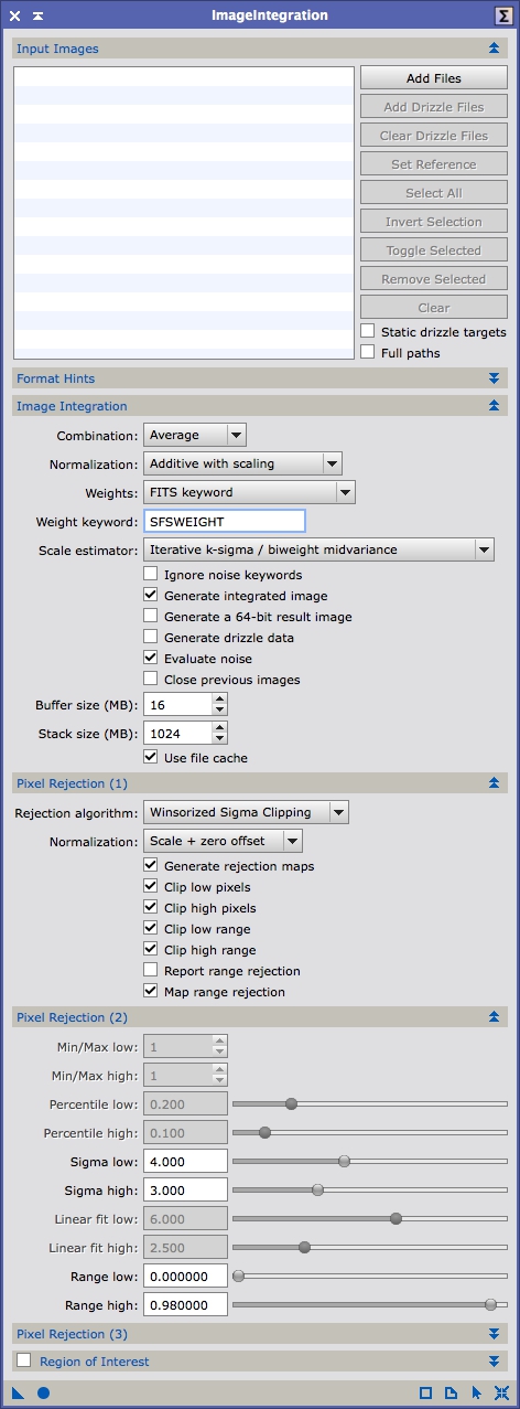
Figure 18: ImageIntegration

Both the rejection maps can be useful.  The rejection_high can show you how well satellite trails or other spurious data has been rejected.  If the image is starting to look almost grey or white you are throwing out too much data.  The rejection low frame can show you low signal areas typically from drift in the image whether intentional (dithering) or not (differential flexure or polar misalignment).  You may also want to monitor the output of ImageIntegration in the Process Console.  It will show you exactly how many pixels are being rejected in each frame how it is weighted, etc.

Again, if you are imaging with a monochrome camera you will need to integrate each filter separately, which means running ImageIntegration multiple times.

This manual process seems very time consuming and complex, but the results you can get are worth it.  You can also speed things up by saving off your typical settings in process icons (see Figure 19).  Once you have the flow down it goes fairly quickly.

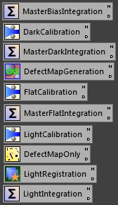
Figure 19: My manual process icons

The best results I’ve gotten out of manually processing my data showed a decrease in average FWHM of 15.3% (3.45″ stars down to 2.92″) with almost no change to the SNR of the final stack (I measured a 0.1% decrease) when compared to the output of BatchPreprocessing.

Good luck processing your data and I hope this helps you get the most out of it!

 

Refrences

Information on calibration frames:

http://www.pixinsight.com/tutorials/master-frames/index.html

Information StarAlignment:

http://pixinsight.com/doc/tools/StarAlignment/StarAlignment.html

Information on ImageIntegration:

http://pixinsight.com/doc/tools/ImageIntegration/ImageIntegration.html