This is another tutorial spurred on by a Cloudy Nights discussion.  I posted this same tutorial in pieces on that thread but decided to duplicate it here.  Thanks very much to Eric Weiss, who provided the M42 data for this tutorial.

The first thing I do when I bring up any raw data is to use the ScreenTransferFunction auto stretch feature. This is a non-destructive process. It simply modifies how the image is displayed and does not alter the data itself. This is really great and allows you to get the data in linear form longer. You can access the STF auto stretch from the menu bar and from a dedicated tool. The radiation like symbol is the auto stretch button. The linked chain icon locks the RGB channels to the same stretch, so if your data is not color balanced then it is best to turn this off before stretching, which is what I did for Mostlyeptyspace’s data.

Figure 1: The STF functions on the menu bar

Figure 2: The STF Tool

So the first thing I noticed when I brought up Mostlyemptyspace’s Orion Nebula data is that there are low signal areas. These occur when there is some amount of drift over the total exposure time. This could be intentional, from dithering between frames, or unintentional due to differential flexure, polar mis-alignment or unguided imaging. Before we do anything else we need to crop the image to include just the higher signal area. This is usually obvious in PixInsight when we have the ScreenTransferFunction auto stretch applied to an image. The STF tool allows you to stretch the image so the data is easily visible without modifying anything. It is a display only function.

To crop the image you can use the DynamicCrop tool, the Crop tool or if you are feeling very brave you can even use PixelMath, but for our case DynamicCrop is the easiest to use. Simply launch the tool, either go the Process Explorer and double click on it or go to the Process Menu and click on it there. Once the tool is active if you click and drag in an image window it will create the boundaries for the crop.

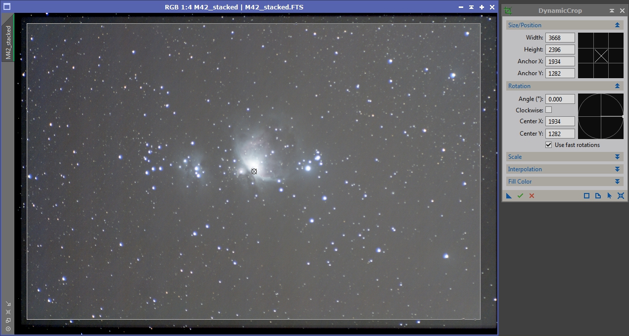
Figure 3: Croping the image

After we’ve cropped the image we can see that there are some gradients and banding visible. The first thing we I’m going to do is go after the gradients. The banding we can remove with a script later on. Bring up the DynamicBackgroundExtraction process and click on your image. I generally start by changing the samples per row setting to give me quite a few sample point and then click on the Generate button. Once I have a bunch of sample I review their placement and make sure that none are placed on stars or on nebulosity. If any samples are coving something other than background either shift it to the side or delete it. Generally I set the correction method to ‘Subtraction’ before executing the process. After all the samples look good click the execute button (green check mark). This will give you two new images, one is the model of the background the other is the modified image. After reviewing the output make any modifications to the samples you feel necessary, close the new images and try it again. Once you are comfortable with the results, check the ‘Discard background model’ and ‘Replace target image’ and execute the process again. This will update the existing image. Because the background has shifted, you will probably need to redo the STF stretch again. Depending on your data it may look worse after the STF stretch as gradient removal allows more of the data, and its associated noise, to be seen. Also, you will likely be able to link the RGB channels now since during the subtraction process the background levels will be normalized.

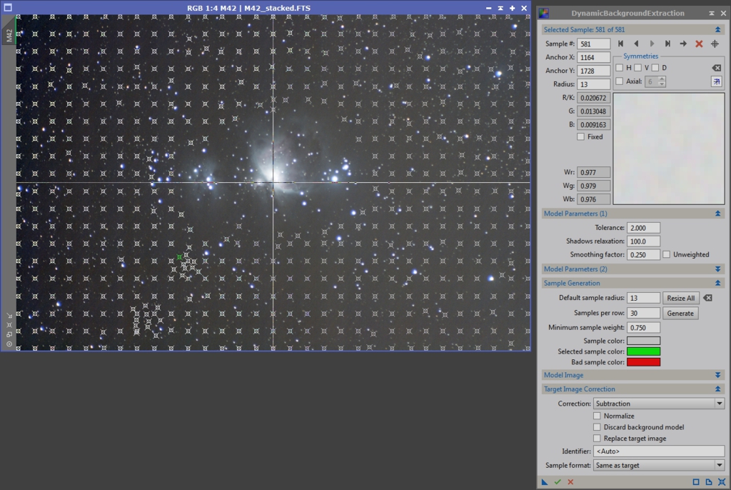
Figure 4: DynamicBackroundExtraction

This particular image was taken with a DSLR and has some banding left over after calibration. This can happen due to gradients present in the light frame data that are not in the calibration data. Light pollution, the Moon and your neighbors flood lights can all create gradients in your light frames that throw off your flat calibration. Since some of these same patterns are in the flat frames the gradient will throw the calibration off. Luckily there is a PixInsight script called CanonBandingReduction that does this amazingly well. It is designed to work on horizontal banding so we first need to rotate the image. The way I chose to do this is by going to the Image->Geometry->Rotate 90° Clockwise menu item (there are other tools to do this as well). Next bring up the CanonBandingReduction script. I didn’t change any of the settings and just hit OK. After this is done, rotate the image back. At this point the background should be looking fairly even. With this image, there is some streakiness left over which we will try to kill with noise reduction. Sometimes doing the CanonBandingReduction can cause or expose additional gradients. This was the case with this data so I went back and did another pass of DBE.

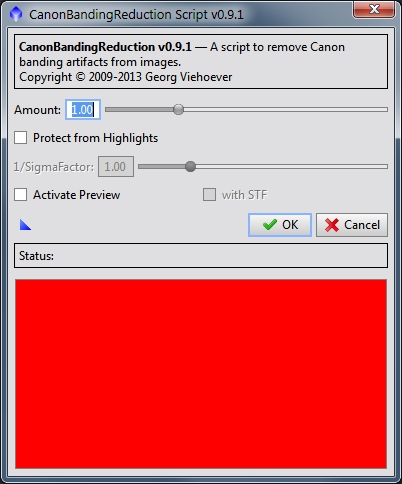
Figure 5: CanonBandingReduction

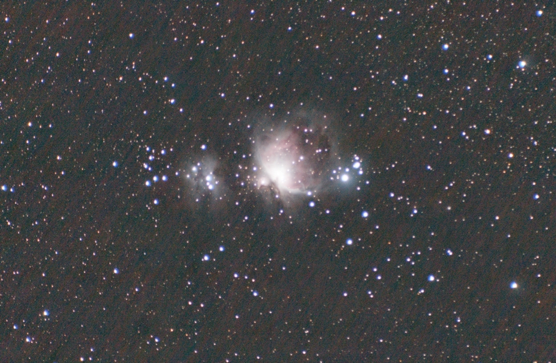
Figure 6: Where we are at after DBE and CanonBandingReduction

Next we are going to prep some masks for other processing. The first mask I will call a light mask, which is essentially just the luminance data from the image with a STF stretch permenantly applied. Go to Image->Extract->Lightness (CIE L*). Apply a STF auto stretch to it. Next drag the triangle icon (New Instance) from the STF window the bottom bar of the HistogramTransformation window. Drag the triangle icon from the HistogramTransformation window to the luminance image. This applies the STF stretch permenantly to the image (make sure to clear the STF stretch otherwise your image will appear all white even though it isn’t).

After we make the light mask we are going to use it make a star mask. Bring up the StarMask process and for running on stretched data we will need to modify the default values. This takes some experimentation and in some cases you may need to use different scale values to catch all the stars, which is the case with the Orion area. For the first pass I used the settings in Figure 7 and applied it to the light mask. Figure 8 shows the second pass, also applied to the light mask. I had problems getting the Trapezium stars to show up when using the light mask, so instead for the last pass I used the settings in Figure 9 and applied it to the main image.

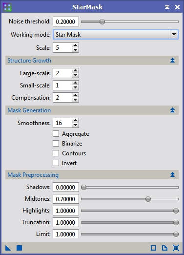
Figure 7: First Pass StarMask

Figure 8: Second Pass Star Mask

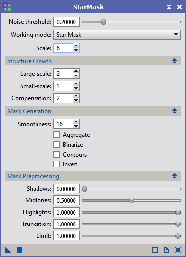
Figure 9: Third Pass Star Mask

We need to make one star mask out of these and the best option I’ve found is to take the max of all the images. Bring up PixelMath and enter this equation into the RGB/L field: max(star_mask, star_mask1, star_mask2) then apply it to the original star_mask image.

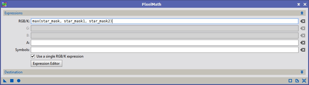
Figure 10: PixelMath Max of star masks

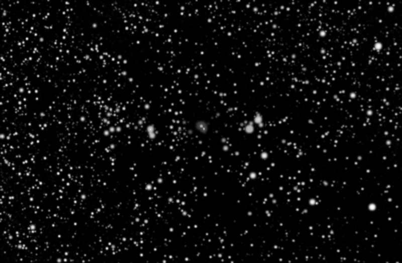
Figure 11: The Final Star Mask

Next we are going to make some copies of the light mask to be used for deconvolution and noise reduction. Make 3 copies of the light mask by draging on the tab in the left bar to somewhere on the PI desktop. Rename them: deconv_mask, tgv_mask and mmt_mask.

Masks are used to protect certain parts of an image when manipulating it. The brightest parts of the mask allow the image to be altered while the dark parts protect it. For example, if you want to do noise reduction but don’t want to affect the stars or brighter parts of your image you can take the light mask and apply it to the image. In this case the mask is actually opposite of what we want, so we can invert it with a click of the ‘Invert Mask’ button which is on the menu bar (or through the Mask menu). You can also enable or disable the visibility of the mask so you can see what’s happening to your image while processing it with the ‘Show Mask’ button.

Let’s start on the deconvolution mask. Normally when I do deconvolution I use the light_mask without modification, but for this image it was difficult to control the effects so I decided to reduce the brights of the mask. In this case I simply cut the histogram range of the image in half, so instead of ranging from 0 to 1 it now ranges from 0 to 0.5. I used the CurvesTransformationTool and clicked on the upper right end point inside the histogram displan and drug it down to 0.5 (See Figure 12). Apply this to the deconv_mask image and you will see it get darker.

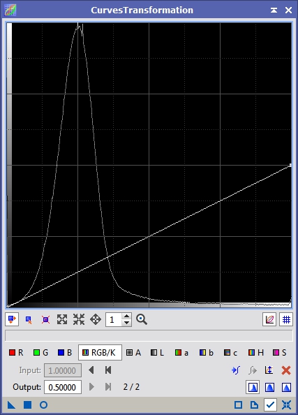
Figure 12: Decreaseing the range of the deconvolution mask

We are going to do something similar for the TGV mask. In this case I want to compress the range from the top and bottom. TGVDenoise can use an image for support, but I find that restricting it’s application to our image is useful. I want to protect the bright portions of the image more than the darker parts but not by too much which is why I compress the range of the mask. Figure 13 shows the CurvesTransformation window before applying it to the tgv_mask window. After this I want to shift the peak of the histogram to the mid point. I used the HistogramTransformation tool with a change to the midpoint and applied it to the tgv_mask (see Figure 14). When used with the TGV process this will give us close to a 50% blend between the original image and the noise reduced image with a slight preference to more NR data being allowed for the background than the high signal areas.

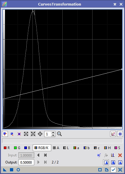
Figure 13: Modifying the TGV mask

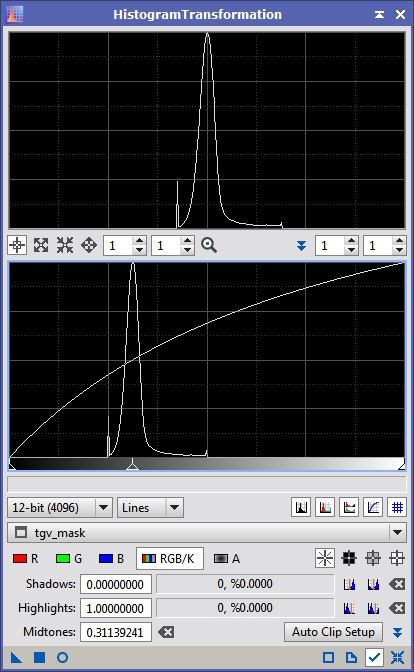
Figure 14: Further modification of the TGV mask

I also use the MultiscaleMedianTransform for large scale noise reduction. I use very aggressive settings for this tool so our mask needs to be very protective to keep more of the original image. In this case I just want to shift the midpoint of the histogram up quite a ways. I usually center it around the ¾ mark, but sometimes go all the way to the 7/8 mark. Use the HT tool as showin in Figure 15 and apply it to the mmt_mask.

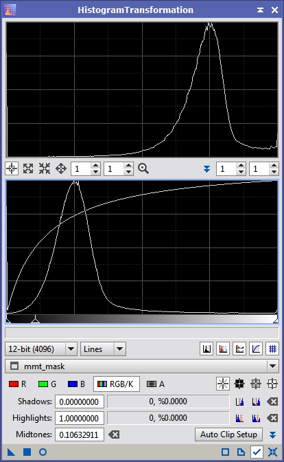
Figure 15: HistogramTransformation modification of the mmt_mask

We are almost done with support images, but we need one more. For deconvolution to work best we need to measure the point spread function (PSF) of the image. The PSF will tell the deconvolution process how the image was convolved. Since stars are point sources and only cover more than one pixel because of how our atmosphere and optics distorts the light we can measure them to try and undo some portion of that blurring. Bring up the DynamicPSF process and start clicking on stars in the main image. For each star you click on you will see a green box show up in the image window as well as some data fill out in the DynamicPSF window. You want to select a range of stars across the image. Pick varying brightness levels, but if you see any stars show up as Gaussian models delete them. The Moffat equation is a better fit to the actual profile of stars and usually the tool will only give you a Gaussian model if the star is over exposed or is possibly a galaxy or other nebulous structure. Figure 16 shows the DynamicPSF window after I’ve selected several stars.

Figure 16: DynamicPSF

Next select one of the lines in the DynamicPSF window then hit CRTL+A to select all of the star data (or you can shift click). Click on the camera icon which will generate a synthetic PSF based on the data provided. For some reason the PSF generated by this can have the wrong size. In my test it was way off and generated a PSF of 13251 x 13251 pixels. We need to crop that down to a proper size and adjust it. Click on the Sigma icon next. This will pop up a window with information about the PSF. Click on the camera icon in that window and it will generate an appropriately sized PSF, however this model is not correct in terms of its rotation. Close the Average Star Data window and bring up the Crop process. Select the PSF view from the drop down menu and then in the target px field put in the width and height of the second PSF we generated (from the Average Star Data). You can get the size information by clicking on that image and looking at the bottom bar of PI. In this case my PSF1 image had a width and height of 27. Put those values into the Crop tool and apply it to the PSF window. You can close the DynamicPSF window and PSF1 image. We need to make one last modification to the PSF image though. The original PSF was normalized and when we cropped the image we messed that up some, so we need to re-normalize it. Bring up the HistogramTransformation tool and if it is not tracking the active window select the PSF view from the drop down list. Click on the ‘Auto zero shadows’ button (it’s on the the Shadows row just past the clipping readout) and then apply it to the PSF image.

We should now a large set of support images as shown in Figure 17.

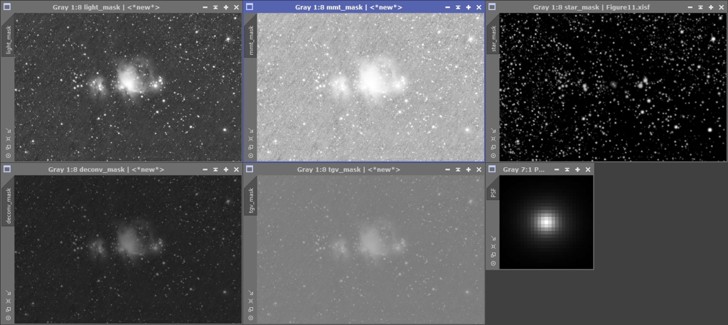
Figure 17: The support images

Now that we have all these support images, lets get on with the next step, which is deconvolution. I do this before noise reduction because those processes can destroy the PSF of stars and we’ll end up with weird effects, like ringing, around them. Bring up the Deconvolution process and click on the ‘External PSF’ tab. This tells it to use an image as our PSF. Select our PSF view by clicking on the ‘select view’ icon next to the ‘View Identifier’ entry field (or you can just type it in). You should show the PSF image show up in the form now. We aren’t going to change too many values for our first attempt but we can go head and set the Deringing options. Make sure Deringing is on and then run your cursor around over the background of our main image and watch the R, G & B values in the bottom bar of PI. For my data these hover around 0.002. You can also use the statistics tool and take the median of the image, but four our first pass this should be good enough. Put that value in as the ‘Global dark’. Leave ‘Global bright’ at zero, turn ‘Local deringing’ on and select the star_mask. At this point your Deconvolution window should look something like Figure 18.

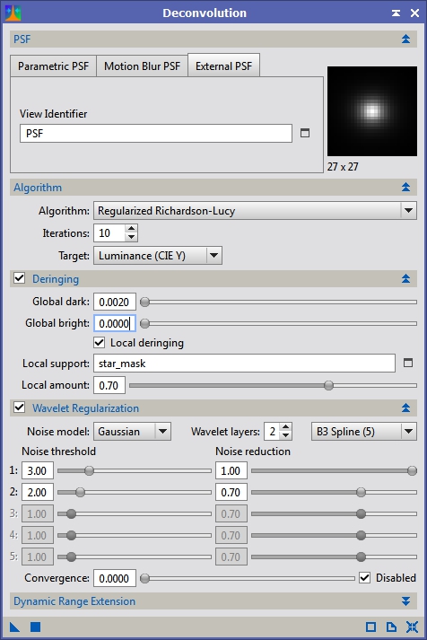
Figure 18: Deconvolution first pass

Before we apply this to our image we need to protect it with our deconvolution mask. Drag the identifier from the left bar of the deconv_mask window to the left bar of the main image (you can drop it anywhere on the bar except over the other images window). This will apply the mask to that window and you will see the image turn mostly red, with the core of M42 slightly exposed. We want to hide this so we can see the effects of the deconvolution process, so click on the ‘Show mask’ icon on the menu bar. To speed things up, lets create a preview window inside our main image that we can run tests on. Click on the ‘New Preview Mode’ icon on the menu bar (also accesible under the Preview menu) and drag a small window around a portion of M42. I made sure to get some of the dark nebula, the Trapezium area and some of the fainter nebulosity. My preview window ended up being around 500 x 500 pixels. You can click on the preview on the left bar of the image window and also go back to the main window. Whatever we do to this preview will be non-destructive so we can test our deconvolution process on it before running it on the full image. Go ahead and apply the Deconvolution process to the preview. Move your STF adjustment around to see what is happening at different levels and then play with the setting in Deconvolution. Keep playing with it until you get setting that you like and then apply it to the main window. Figure 19 shows the final settings I used.

Figure 19: Deconvolution

Now we are going to do some noise reduction to clean up the background. Apply the tgv_mask to our main image and this time invert it using the menu bar or mask menu. I extended my preview to cover a bit more of the faint nebulosity and background for this next round of experiments. Bring up the TGV process and turn on the ‘Local support’ option. For the Support image specifiy our light_mask view. Leave the other settings at defaults in this section. Because I want to do some Luminance and Chrominance noise reduction I switch to CIE L*a*b* mode and turn on both the Lightness and Chrominance tabs. I usually start with fairly small values when working with linear data. Figures 20 and 21 show the settings I started with. Apply this to your preview and see what happens.

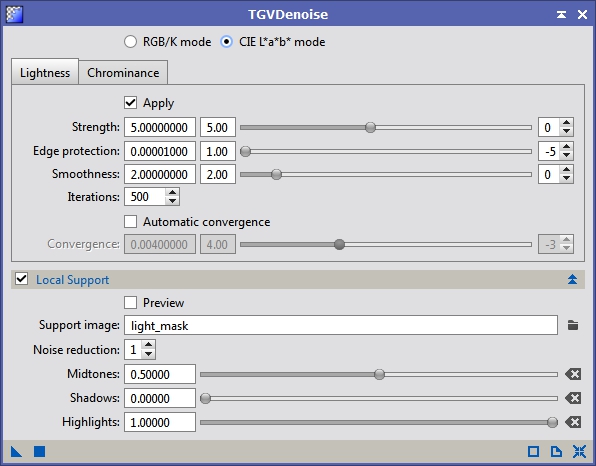
Figure 20: TGVDenoise – Lightness

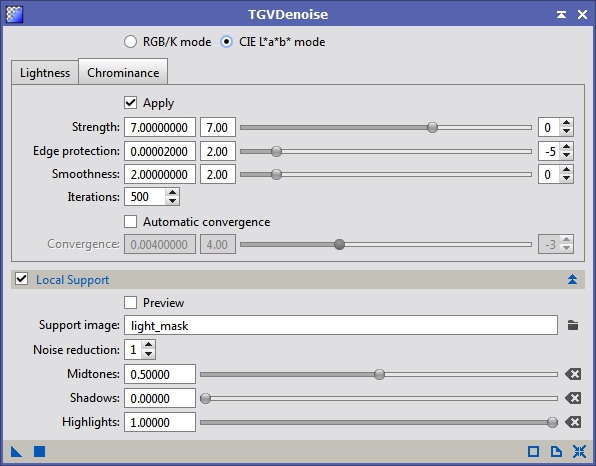
Figure 21: TGVDenoise – Chrominance

Play with the settings some and see what happens each time. I generally don’t touch much besides the edge protection setting but feel free to see the effect of each slider. Once you like your results apply it to the full image. I felt my initial guess was pretty lucky this time and I saw a good reduction of noise in the background without much modification to the higher signal areas.

TGVDenoise is fantastic at high frequency noise reduction (pixel to pixel variation) but not great with large scale structures. This sometimes leaves you with the dreaded ‘orange peel’ effect on your background (also sometimes called mottling). To reduce this we are going to use the MultiscaleMedianTransform process. Go ahead and bring it up and populate it with the values in Figure 22. Apply the mmt_mask to our main image (don’t forget to invert it) and then apply the MMT process to it. This runs much quicker than TGVDenoise so I don’t typically run it in a preview.

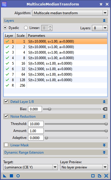
Figure 22: MultiscaleMedianTransform – for luminance noise reduction

The first pass of this looked good, but I still saw a fair amount of the streaking. I ran the same process again and it started to look a bit better. The remaining streaking looked to be primarily with the red color so I stopped here for Luminance. Keep the MMT window open though.

Now we are going to do some large scale chrominance noise reduction. Switch the target in the MMT window from Luminance to Chrominance. We want a more permissive mask for this so apply the light_mask to our main window and invert it. Now run the MMT process again on our main image. You should see the background even out quite a bit more and look more of a nuetral grey than a blotchy red. I wasn’t entirely satisfied with what the background looked like so I did one more pass of MMT for luminance and chrominance, each with the appropriate mask (mmt_mask and light_mask respectively). I now hade an image that looked like Figure 23.

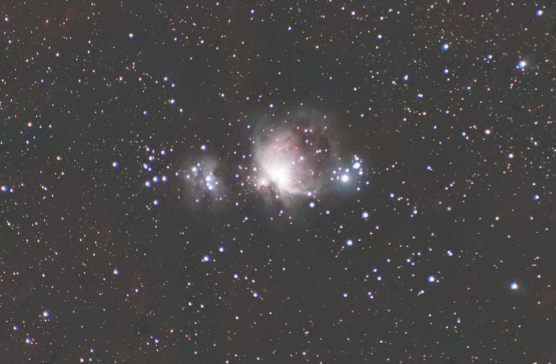
Figure 23: Main image after deconvolution and noise reduction

By the way, if you do a STF on your image now it will look horrible. This is because the background noise has been compressed so STF thinks it can stretch the image a lot more.

Next we are going to stretch the image. Clear any STF stretch on the window and bring up the HistogramTransformation tool. I’ve used the MaskedStretch process in the past but in the case I felt it flattened the image too much but feel free to give it a try. You can click on the preview icon to see instantaneous results of your stretching. Play with the settings in the HT tool and then apply it to your main image. I used the settings in Figure 24 and ended up with the image in Figure 25.

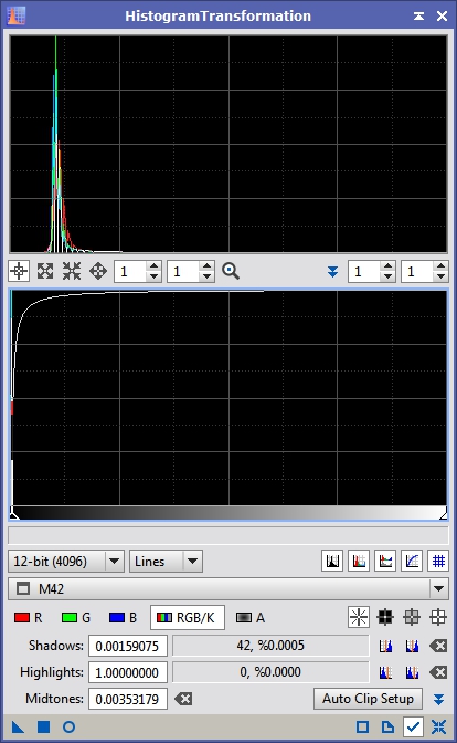
Figure 24: HistogramTransformation – initial stretch

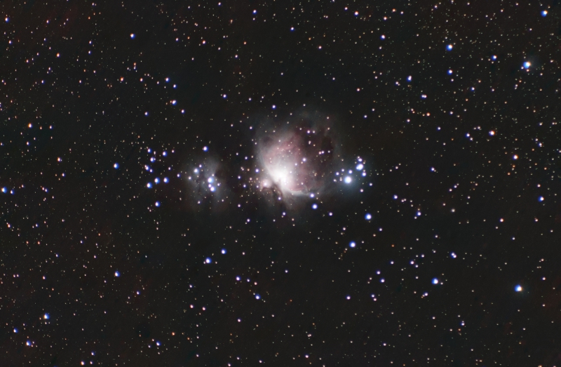
Figure 25: Resulting image after stretch

Now, lets do some HDR to bring out the core of M42, which is over stretched a bit. Bring up the HDRMultiscaleTransform tool and populate it with the setting in Figure 26. It runs quickly so you can apply it to the full image if you like.

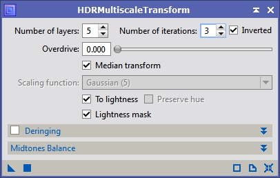
Figure 26: HDRMultiscaleTransform

I found it to be far too aggressive so I think we need an additional mask. Take any one of the other masks and make another clone of it. Rename it to hdr_mask and then bring up the PixelMath process. Put the value of 0.25 in the RGB/K field and then apply it to our new hdr_mask image. This will replace the entire image with the value of 0.25.

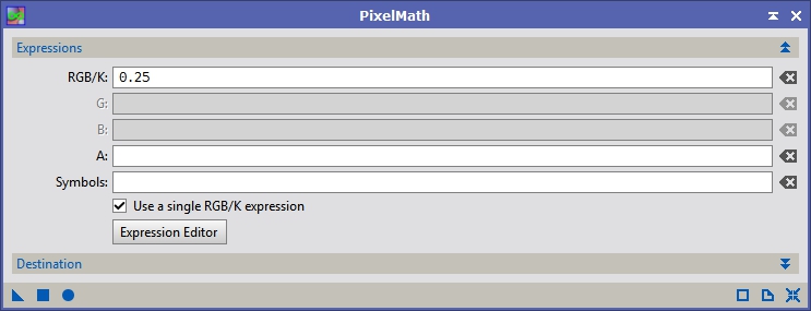
Figure 27: PixelMath – grey mask

Now apply that mask to our main image and try the HDRMultiscaleTransform tool again. That should look much better. The Trapezium area should now be visible at the same time as the fainter nebulosity.

Next we are going to enhance some of the structures a bit. Bring up the LocalHistogramEqualization tool and remove the mask applied to the main image. This tool increased the contrast between structures of particular sizes. For example the dark lanes in galaxies along with the star forming regions in the arms will get darker and brighter respectively. This is a great contrast enhancing tool. I did one pass with a strucure size of 64 (see Figure 28) and another of size 24 (see Figure 29). After this you should have an image that looks like Figure 30.

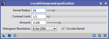
Figure 28: LocalHistogramEqualization – first pass

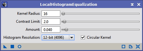
Figure 29: LocalHistogramEqualization – second pass

Figure 30: Image after HDR and LHE

Next on the list is reducing the color halo-ing around the stars. Apply the star_mask to our main image then bring up the CurvesTransformation tool. I tend to like my stars fairly white so I’m going to be very aggressive with the saturation reduction to hide the color outside the edge of the stars. Figure 31 shows the curve I applied to the image. Since the star mask is in place we should only see the stars loose saturation.

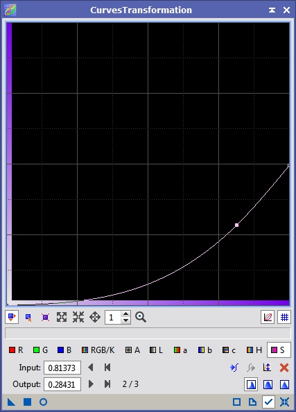
Figure 31: CurvesTransformation – star saturation reduction

After trying to increase the saturation of the rest of the image it looked like we needed another mask, so I duplicated the light_mask and renamed it sat_mask. Then I applied PixelMath to it with the settings in Figure 32. This removes the stars from the light mask so that when we increase the saturation it won’t increase the star color at all. Apply this new mask to the main image.

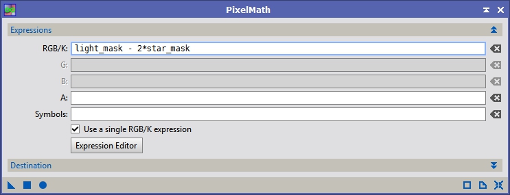
Figure 32: PixelMath – saturation mask

Now lets boost the color. Bring up the CurvesTransformation tool again with the settings in Figure 33. Again experiment to see what you like best. Apply this to the main image and watch the colors pop.

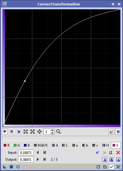
Figure 33: CurvesTransformation – boosting saturation in the main image

Now we are finally done! You should have an array of images that should look something like Figure 34 and a final image that looks something like Figure 35.

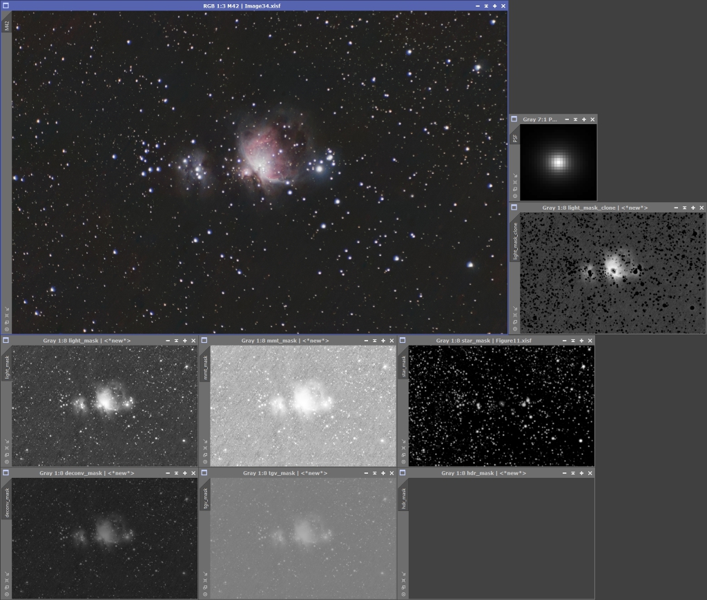
Figure 35: The final image along with all support images

Figure 34: The final image