Clouds, horrifically bad seeing, rain, oppressive heat, the Moon and of course a regular day job. These are all things that can keep you from heading out to do some astrophotography. Over the last year (about 7 and a half months as I write this) I managed to go out and acquire some data 36 times. Compare that to 2 years ago when I was able to go out 54 times. I don’t know if 2012 was a fantastic year and the last two are normal for Central Texas as I’ve only been imaging for a little over 3 years, but it seems the weather has simply not cooperated with me recently. Work has a lot to do with it as well. I have an entirely mobile setup and it takes a couple hours to pack everything up, drive to my normal imaging location and setup my equipment. Then it takes another hour to break down, drive home and unpack everything. That overhead makes it very difficult to get more than an hour or two of imaging in on weekdays during the summer and there have been very few clear evenings on the weekend this year. This may sound like a general rant, and of course it is, but there is a point to be made here. I’ve had a significant number of days this year where I really wish I could be out imaging and just can’t because weather, work and the phase of the Moon don’t line up.
Given the extra time on my hands I started wondering if could I be working on my processing skills while I’m stuck indoors. I could go back and reprocess some of my older data to see if any more could be extracted from it but a new idea came to me while trying to help others with their imaging project. I have a friend, a doctor of astrophysics, who teaches physics at a local college and they have a small observatory. He had some students that were helping him with a research project he was involved in and in addition to the data they were required to take they also wanted to capture some pretty pictures of M104 and M51. Being the nice guy that he is he gave them some time on the scope. They collected data over multiple nights and before they left for the summer I sat down with them to help turn their data into images. The complication was that the research scope does not use standard RGB filters. It is an older setup and uses the Johnson filter set. The blue band filter in his particular set is very restrictive so they tend to avoid using it and do most of their data acquisition with V, R (they do have a luminance filter as well but it is not used frequently for research).
A pseudo blue channel can be constructed by subtracting some portion of the V & R data from L, but their L data was very poor due to heavy light pollution in the area (and frequently Moon light) causing flat correction issues. I decided to see if I could make a pseudo color image from just the V & R data. Before I sat down with them to process their data, I wondered if there was a source of data I could use to practice and try out some blending methods. In fact there are several resources available online but the one I found most appealing was the Sloan Digital Sky Survey. You can probably tell from the name, but the SDSS project uses Sloan filters. These are more permissive than the Johnson filters with sharper cut-offs but the principle should be similar. I did some spreadsheet calculations to determine how much area is under the related curves of Sloan g & r filters vs Astrodon RGB (I did similar studies on the Johnson filters). Because the overlaps are not 100% there is some unaccounted energy that throws the color balance off but as we’ll see later this can be corrected.
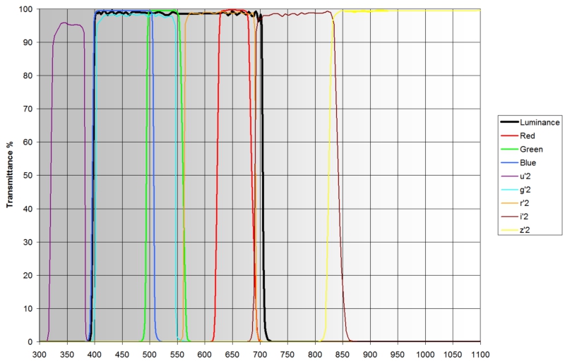
Figure 1: Astrodon LRGB vs. Sloan
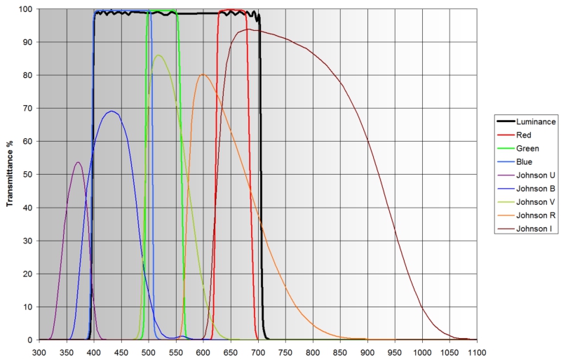
Figure 2: Astrodon LRGB vs. Johnson
You can see that the Sloan g filter almost entire covers the B and G bandwidth of the astrodon filters. This makes it nearly impossible to separate them, but due to the nature of astronomical objects this isn’t much of an issue. Objects tend to be very blue due to the light from bright blue stars or a cyan color from the light emitted by ionized oxygen. So from this perspective if we come up with an equation that modifies the green channel based on the g and r data we might end up with an image fairly close to ‘true’ RGB. What I found works best is the Average Neutral Protection method described in the Subtractive Chromatic Noise Reduction section of the PixInsight documentation. This takes the minimum of the of the pseudo green channel and the average of the pseudo red and blue channels. The idea of this filter was to remove background green noise from OSC and DSLR cameras but keep the green channel of the objects and stars in the image protected. In our application it works wonderfully at shifting the cyan color to more of a true blue for galaxies and reflection nebula. Planetary nebulae tend to be shifted slightly to the blue as well, although this can be corrected some by playing with the ratios in the PseudoG calculation.
Based on the Astrodon RGB vs. Sloan I’ve come up with this set of equations to make an psuedo RGB image. The values use see in the equations are based on the relative areas of the v, g & r filters compared to the Astrodon R, G and B:
PseudoR = r
PseudoB = g
TmpG = 0.976867918*G + 0.023132082*R
PseudoG = 0.4*TmpG + 0.6*min(TmpG, (r + g)/2)
Similarly these are the equations for the Johnson filters:
PseudoR = 0.292901909*V + 0.707098091*R
PseudoB = 0.995890089*V + 0.004109911*R
TmpG = 0.872704584*V + 0.127295416*R
PseudoG = 0.4*TmpG + 0.6*min(TmpG, (PseudoR + PseudoB)/2)
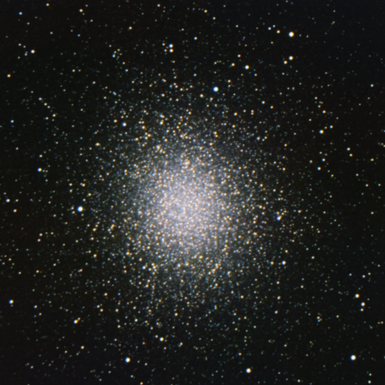
Here are some example images from the SDSS-III data. There is minimal processing on these images (although most of the images are mosaics). I’ve done a linear fit between g & r data before combining into an RGB. A non-linear stretch was performed to make the objects visible on a monitor. The saturation was pushed a bit to bring out the color more. After saturation boosting I did a color balance (background leveling and white point based on image statistics) and then resized them for the web:


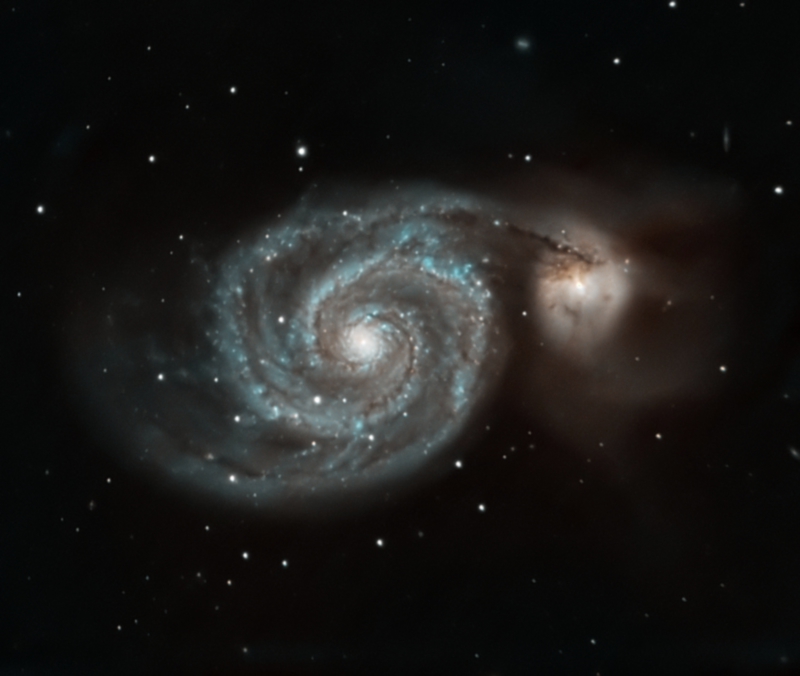
For the Johnson filters, here is M51 using the students data. I’ve done much more processing to this as it was significantly more noisy than the SDSS-III data but I did use the equations mentioned above for generating the color image:
I felt like my processing of the students data was a success and in the process of preparing to work with them I realized there are lots of scientific resources out there who’s data is freely available to play with. This has really helped me keep my eye in with image processing and at the same time I’ve been able to examine some fantastic objects several of which I will probably image myself in the future. So, when the clouds are hanging around for months at a time, download some data from the SDSS repository and have some fun.
I hope you find this fun and useful!