There are many ways to approach the purchase of a camera for astrophotography. You may already have a scope that you want to pair a camera with or you may be looking for purchasing both together. Or maybe you’ve gotten started with imaging already and you want to improve your results but don’t understand the interaction of camera and scope. The purpose of this tutorial is to describe the properties of scopes, cameras and everything in between to help you choose or improve your setup. One additional note before we get into it, this article is geared towards long exposure astrophotography. Planetary imaging is a different beast and the needs of each type of setup tend to be very different. As I don’t have a lot of experience with planetary imaging I will leave that topic to others.
Before we even get to cameras and scopes, let’s talk about mounts. Your mount is the most important part of your entire setup. If your mount is not capable of tracking your target accurately with the load of your imaging equipment then the best camera and scope in the world will not help you to get good images. That being said I will leave the topic of mounts for another tutorial.
To get things started, lets discuss how CCD and CMOS sensors work. Both technologies rely on the photoelectic effect to generate photoelectrons which are stored in capacitors (the well) as charge. The main difference between CCD and CMOS sensors is how that charge is interpreted. The pixel’s charge wells are coupled which is why the name charge coupled device or CCD. The charge is shifted to adjacent pixel towards a read-out register one row at a time. That read-out register then shifts the charge one pixel at a time to an amplifier and A/D (analog to digital converter) which turns it into a digital value (see figure 1). CMOS sensors have an amplifier and sometimes A/D at each pixel. This allows the chip to be read much faster as you can read all pixels at once. The additional circuitry at each pixel as two major effects. It decreases the amount of photodiode area for a pixel since the circuitry itself takes up space. Since no two amplifiers or A/Ds are exactly the same the read-out of each pixel will vary causing uniformity differences. These two reasons are why CCDs are typically preferred for astronomy instead of CMOS sensors (although modern CMOS sensors have decreased the impact of both of these issues dramatically over the years).
Figure 1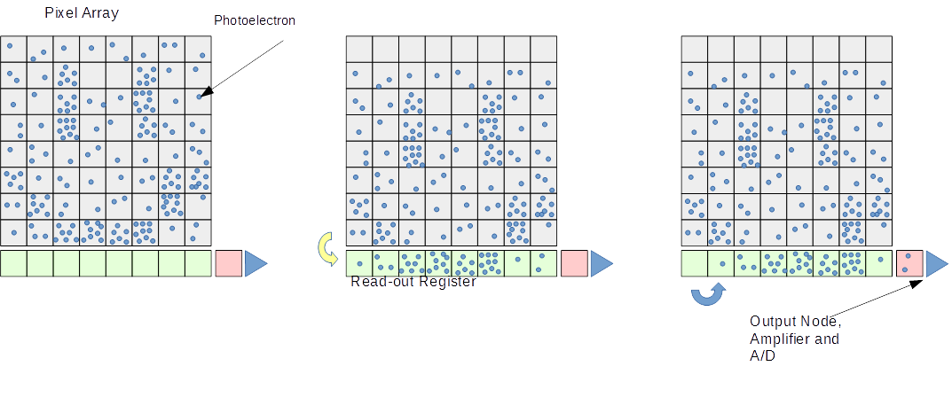
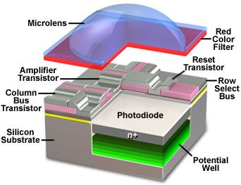
Both CCD and CMOS can be manufactured with filters and microlenses. The filters limit the frequency of light each pixel receives (usually in the form of an RGB bayer matrix). The microlenses sit above the filters and focus light towards the photodiode area increasing the light gathering capabilities of each pixel (see figure 2).
Figure 2
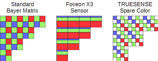
Most CMOS sensors use a bayer matrix with two green pixels, one red and one blue. These are then interpolated to make a full resolution color image. Technically some resolution is lost because each color pixel is separated by another color although the bayer interpolation algorithms due a good job of regaining a lot of that resolution. Figure 3 shows a standard bayer matrix along with some other topologies used by specific sensors.
Figure 3
You can also make color images by placing a filter in front of the entire sensor (see figure 4). A lot of astrophotographers use this arrangement as you can utilize the full resolution of the sensor and can use other filters besides RGB, like Hα (which only passes light emitted by excited ionized hyrdogen atoms).
Figure 4
CCD and CMOS camera have intrinsic properties which affect the overall image quality you can achieve. I won’t try to tell you which is most important because that will vary based on your needs, but I’ll try to detail exactly how each characteristic affects your results. The properties I’ll discuss are: quantum efficiency, linearity, read noise, dark current, well depth dynamic range and gain.
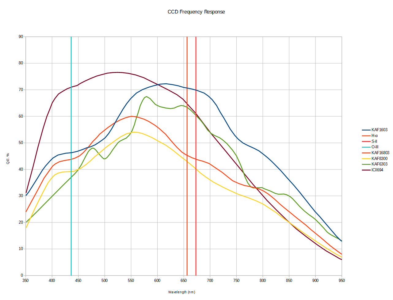
First, let’s talk about quantum efficiency. Ideally each photon that strikes the photoactive region of a pixel would be converted to a photoelectron and stored in the well. This is unfortunately not the case. Most sensors have a peak efficiency below 80% and the efficiency varies based on the frequency of the light falling on the sensor. For example, the Kodak KAF-8300 sensor has a peak efficiency of around 55% which falls to about 43% at the Hα frequency. Figure 5 shows the response of several common CCD sensors. If you are looking at one-shot-color (OSC) cameras keep in mind that the bayer matrix will most likely not be factored into the efficiency data provided by the manufacturer.
Figure 5
Linearity is the measure of how close a sensor tracks the conversion of photons to to photoelectrons. If you normally get 1 photoelectron for every 2 photons you want that to continue as charge is built up. If you’ve filled up 3/4’s of the well and you start to get 1 photoelectron for every 3 photons then your image data is no longer linear. This means that brighter objects in your image will appear less bright than they truly are. In general, I wouldn’t say this is terribly important if your goal is only to take pretty pictures. However, if you plan on doing any science with your equipment then this is much more important.
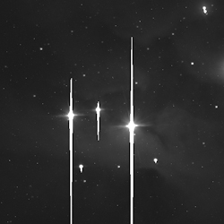
Most cameras designed for amateur astronomers have anti-blooming gates (ABG). What’s that you ask? Have you ever seen an astronomical image like figure 6? The vertical lines are blooming. This occurs in CCDs when the light focused on a pixel is so bright the charge builds up and overlows its own well spilling into adjacent pixels. Charge coupled devices are typically only coupled in one direction giving the photoelectrons only one path to flow (the same path they would normally be read-out in). In figure 6 it’s clear the charge coupling is vertical. Anti-bloom gates bleed off the charge as it gets close to the maximum the well can hold. It’s the anti-blooming which tends to cause non-linearity. When an ABG sensor becomes non-linear varies from one to the next. So, if you want to use it for scientific purposes you will need to measure the linearity of your sensor and make sure that your subject data does not peak above that limit. Non-anti-blooming gate (NABG) cameras are also available if your primary goal is scientific work like photometry.
Figure 6
Read noise refers to the noise associated with reading the chip. It is typically measured in electrons or e-. There is a fixed pattern and random element to scanning the data stored in the sensor and converting it to a digital signal. This occurs for a couple reasons. Converting the analog charge to a digital signal via the amplifier and A/D is not 100% accurate. If you passed the same electron charge through the same circuits you would get different digital values, although they would all be very close to the ‘true’ value. The surrounding electronics will also affect the charge passing through the entire system. The fixed pattern from these noise sources can be removed with bias frames (I’ll discuss image calibration in another article) however the random element can only be reduced by stacking multiple frames (this is true of any random noise). You can also swamp the noise with signal. This is why daytime photography doesn’t typically do any image calibration. This signal charge is so much larger than the noise you can essentially ignore it. Discussing the details of signal to noise ratio would be a little too detailed to include in this article but a side effect of that physics is that sensors with high read noise benefit from longer exposures while sensors with low read noise can get a way with stacking many shorter exposures. In most cases the lower the read noise the better but this obviously needs to be balanced with other factors.
Dark current is a measure of how quickly charge builds up in the wells when no light is falling on the sensor. It is measured in e-/s (electrons per second). Unless they are absolute zero all atoms in a material vibrate with electrons jumping valence bands as energy passes into and out of their local system. The warmer the material the more interaction. Because these electrons from the surrounding material can pass into the well they can be trapped there just like the electrons from our signal making it impossible to distinguish the two. Because this action is highly temperature dependent most astronomical CCDs are cooled. The more the sensor is cooled the less dark current it has (after a certain point other unwanted effects pop up so you can cool too much). This is another case where lower is always better.
Well depth is a measure of how much charge the well can hold. It is measured in electrons (e-). The well is essentially a capacitor and like all capacitors it can only hold some much charge. Process technology and area under the photosite determine the maximum charge so if you had two sensors made with the same technology but one had 4μm square pixels and the other had 8μm square pixels then the larger pixels would hold 4 times the charge. This is one of the CCD characteristics I tend to ignore unless the well depth is exceptionally small because it can be worked around by taking exposures of different lengths and combining them with HDR techniques.
Dynamic Range is inferred from the read noise and well depth (and dark current if it’s very high). In electronics dynamic range is typically measured in decibels. Equation 1 below shows how to calculate it. And if you want to account for dark current you have to estimate your typical exposure time and include it in equation 2. This tells us how much usable charge there is in any given camera. This is a better measurement than just looking at well depth alone since it factors in the bottom limit below which no signal can be distinguished from noise.
Equation 1
![]()
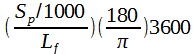
Equation 2
![]()
Gain is the last property and refers to how the amplifier and ADU convert the photoelectric charge into digital values. It is typically measured in e-/ADU (analog to digital units). This is typically set by the manufacturer so that the maximum well depth is near the maximum digital value. Most astronomical CCDs use 16 bit A/Ds giving a maximum digital value of 65535. If you had a sensor with a full well depth was 20,000e- then the ideal gain would be around 0.3 e-/ADU. I know this looks like fractional electrons are being turned into ADU, but really it just means you need over 3 electrons before you increase the ADU by one. This gain would maximize the dynamic range of that sensor. Some manufacturers hide the top end non-linearity of their sensor by dropping the gain some. This means that the ADU will max out before you reach the full well capacity of a pixel. Also, changing the ISO values in a DSLR is effectively changing the gain of the sensor. You can actually measure the characteristics of your DSLR sensor to determine what the gain is at each ISO setting. By increasing the ISO you reduce the dynamic range of your sensor and increase the noise but you get an image of equivalent signal ‘faster’. So if your setup does not allow you to take long exposures then pushing the gain or ISO up can be beneficial (up to a point).
Now that we’ve covered the characteristics of sensors lets talk about field of view and image scale. These are both very similar where field of view describes the area of the sky that your sensor covers with a particular optical setup and image scale is the area of sky that a single pixel covers. There are some really nice tools out there that let you explore different arrangements of optics and cameras. The one I use the most is CCDCalc written by Ron Wodaski. It’s free but is limited to Windows only. There’s an online version here:
http://www.skyatnightmagazine.com/field-view-calculator
I’ve heard there are several apps for iOS and Android as well, but I have not used them. These tools are great for getting visual representation of what a particular system would see but it also helps to understand the math behind them. We’ll talk about image scale first because determining field of view is a simple scale from that calculation.
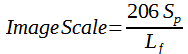
You will usually see the image scale written as equation 3: where Sp is the size of a pixel in μm, Lf is the focal length of the scope and Image Scale is in arc-seconds per pixel (1/3600th of a degree). The value of 206 comes from converting μm to mm and radians to arc-seconds. The exanded form looks like equation 4. Here you can see the conversion of μm to mm by a factor of 1000 next to Sp. Then the conversion of radians to degrees 180/π and finally the conversion of degrees to acr-seconds by multiplying by 3600. If you take (180*3600) / (1000* π) you get approximately 206. Let’s put the equations to use with a simple example. Say I am investigating a camera with pixels that are 5.4μm in each direction (this information is usually available from the manufacturer) and I already have a scope with a focal length of 1500mm. Pairing the two my setup would have an image scale of 0.74 arc-seconds. This is a very small portion of the sky but depending on your environment and mount it may not be unreasonable. If your pixels are square then it will cover the image scale will be the same for both x and y, if not you can separate the two.
Equation 3
Equation 4
The next topic is under and over sampling. This goes back to Henry Nyquist who in 1928 published his theory on sampling telegraph transmissions. It states that in order to accurately measure a signal you need to sample it at twice the rate of the highest frequency in the transmission. When we are talking about frequency with respect to creating an image on a CCD we aren’t talking about the frequency of the incoming light. Rather we are talking about the dimensional scale. For example, when the image is formed at the focal point of the telescope how many arc-seconds does a star profile cover from the peak to the background. The shape of the star profile is similar to a sound wave with a peak and a trough (see figure 7) but in two dimensions.
Figure 7
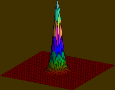
Before we continue, there are two concepts you need to understand. Theoretically, a star’s light should always fall on one pixel, they are so far a way that the angle measure of its surface is multiple orders of magnitude below an arc-second. However, because our atmosphere blurs the image along with the optics of the scope that point source of light is spread over an area. Usually, stars follow a Gaussian, Moffat or Lorentzian equation. This spreading is called the point spread function or PSF (also see Figure 7). Related to the PSF is a measurement called the full width half maximum or FWHM. The FWHM is simply the diameter of the PSF at half of its maximum falue. Think of the circle (or ellipse) that you would see by slicing Figure 7 horizontally halfway between the base and the peak of the function.
There are two things the Nyquist rate inappropriate for our purposes though. First, Nyquist was trying to recreate sine waves with ideal sampling points. If you shift where you sample your signal you won’t be able to re-create the original (see figure 8). Second, because we are sampling across a two dimensional grid we have to account for the longer diagonal across the pixels. Assuming we are using square pixels then the diagonal is 1.414 times longer than one of the short edges. If we use the Nyquist rate then we should sample at 2.828 times the highest frequency. For example, if the smallest PSF of a star that we can achieve with our optics and atmospheric conditions has a FWHM of 3 arc-seconds then each pixel should cover no more than 1.06 arc-seconds of the sky. Assuming we want to account for poor sampling points then that number should be even smaller. For the most part, I feel that using an image scale of 1/3rd the best FWHM you can achieve is good enough. Any improvement in resolution you get after that is very minimal.
Figure 8
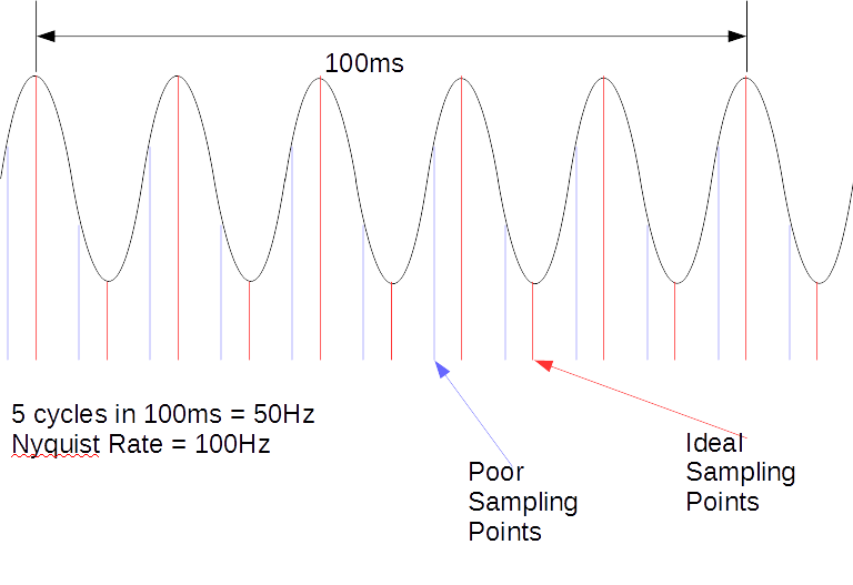
Now that we’ve talked about ideal sampling it should be easy to interpret what under and over sampling means. Under sampling is simply not sampling enough or for our purposes the image scale at the sensor is too large to capture the detail that the optics and atmosphere allow. In cases of severe under sampling the entire PSF of a star fits within a pixel and if you enlarged the image the stars would appear square. Like most things under sampling is not all bad; if you are looking to capture a really wide field of view, loosing some of the finest details my be acceptable. Over sampling is where you sample the signal too much. In our example above if you could achieve 3 arc-second FWHM stars and your image scale was 0.3 arc-seconds then you are sampling too much. Again, over sampling is not the end of the world. On those days where your atmospheric seeing is amazingly good it could allow you to achieve much higher resolution images. Over sampling also reduces the field of view you could achieve when paring the same camera with different optics or conversely paring the optics with a camera that has larger pixels. There is also a signal to noise impact at the pixel level, but this can be mostly regained if you are willing to use the binning feature of most CCD cameras or you re-sample your images later on (true binning is not available on any kind of OSC camera including DSLRs).
We’ve already hit on some environmental conditions like atmospheric seeing, but I’ve kind of glossed over those, so let’s discuss them in more detail to see how they affect what kind of setup you build. The signature in a lot of amateur astronomer’s emails and posts, “clear skies,” refers to the first item on the list: clouds and transparency. Clouds are easily seen and it’s just as easy to see how it would affect your imaging. Some clouds are dense and you can’t see any astronomical objects behind it, some are a little less so allowing some amount of signal to pass. Keep an eye on the weather forecasts can help you plan when to go out. Also, if you log your conditions you can get a feel for your prevailing patterns. How frequently are you clouded out, do your clouds typically disappear after sunset. This will help you gauge the frequency that you can image. Keep in mind that patterns change from year to year. For me 2012 was a great year with 2013 being significantly more overcast. Transparency is related to clouds. This is sometimes related to a high haze but can also be from dust or smoke in the air. It’s usually difficult to spot during the day but at night you will notice that the extinction point for the stars along the horizon is higher up and that fewer stars are visible over head.
Wind can also affect your imaging. If you typically have very high winds then you will either need to be imaging with a very robust mount, a very small short focal length scope, inside a structure like an observatory or maybe all of the above. The wind will push and pull on your equipment and when you are trying to image at very small scales and tracking at even smaller ones it can have a large impact.
Temperature can also affect your session. Never mind the fact that when it’s bitter cold it is difficult to work with your equipment and monitor it through out the evening (the same goes for when it’s blazing hot and the bugs are eating you alive), but it can also affect the grease in your mount the temperature regulation of your camera, the dew point and how dew much accumulates on your equipment. Temperature change is also an issue. The metal in your scope may compress as the temperature drops during the night causing you to refocus more frequently. With larger mirrors and lenses the optics may not stabilize with the ambient temperature causing fluctuations in the image.
Astronomical seeing is causes by our turbulent atmosphere. At higher altitudes the movement of pockets of air shift around in high winds causing lensing effects. As the pockets and air moves the light is refracted in different directions. This will limit the true resolution that you can resolve. In most of the populated world the atmospheric seeing varies from about 2 to 5 arc-seconds. You typically have to get up to higher elevations so that you are looking through less atmosphere to do better. This is why a lot of observatories are built on mountain tops. As we discussed previously, understanding your typical seeing conditions is very useful for determining an appropriate image scale.
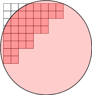
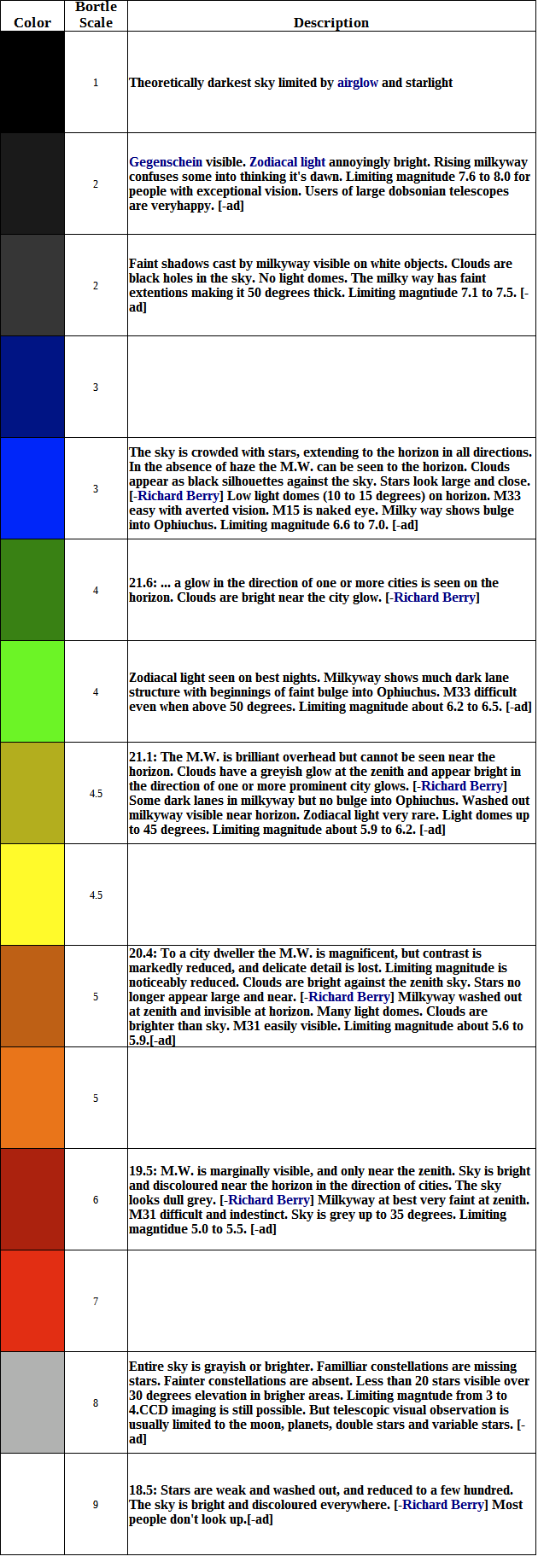
Light Pollution also affects your imaging. As more light is directed into the sky it scatters in your atmosphere causing a brightening of the background. Because this is unwanted signal it can be treated as a straight addition to noise bringing down the overall signal to noise ratio. For example, if I image in my backyard which is in a Bortle scale 7 (See figure 9) and then drive out of town to one of my clubs dark sky sites which is a Bortle scale 4 the signal to noise ratio improves about 5x. Imaging straight luminance or RGB in red zones is difficult. I won’t say it’s impossible to get good LRGB results in light grey and white zones but you will have to have a very patient and dedicated disposition to do this and not start throwing equipment around.
Figure 9
The Moon has a similar effect to light pollution. When it is full and high in the sky the light scatter and gradients across the sky can be severe. Many astro-imagers use the full Moon phase to test equipment, flush out software, process acquired data and sometimes go on the forums and complain 😉
There are several handy websites that help with forecasts, logging your conditions:
Weather Underground (wunderground.com) gives a great hourly forecast so that you can see how the conditions change during the night. Other services lump the entire day into one forecast which isn’t very helpful since it could be cloudy all day but may clear up in the evening.
Clear Sky Chart (cleardarksky.com) is a great service that uses data from the Canadian weather service to predict clouds, transparency, astronomical seeing, lunar phases, temperature, wind and humidity. As all forecasts it’s not 100% accurate but it gives a good indication. The Bortle scale data in Figure 9 was compiled from the the CSC webpage.
Unisys Weather (weather.unisys.com) has some great animated cloud cover and transparency maps. This can help you predict if the clouds sitting over currently you are going to clear out or not.
Time And Date (timeanddate.com) has a nice page for sunrise and sunset that times over a given month.
http://djlorenz.github.io/astronomy/lp2006/overlay/dark.html has the most up to date light pollution map combined with Google maps display so you can estimate what the Bortle scale is in your area or at potential dark sky imaging sites. There are also overlays for Google Earth.
This isn’t a truly environment problem but the optics of your scope also limit what you can resolve similar to astronomical seeing. A scope with 4” of aperture and high quality optics can already resolve more than the atmosphere will allow in most cases. This is why astrophotographers tend to gravitate towards small high quality refractors. To estimate the diffraction limit of a scope in arc-seconds use 115.76/D (D is the aperture of your scope in mm, this also assumes that the frequency of light is 460nm). When optimizing your system for resolution you would use the worst case between the diffraction limit and the average seeing (worst case being the highest number).
Beyond environmental affects there are other things that affect your imaging session but for the most part these are under your control like: polar alignment accuracy, cable management, equipment cleanliness, drivers & software, etc. I’ll discuss these in more detail in another post.
So, that’s a lot of information and pulling all that together to make an informed camera choice is not trivial. Let’s try to boil it down to the nuts and bolts of how to all this information to help you make a decision.
If you are looking to image wide field objects then going for maximum resolution isn’t necessary. Instead focus on maximizing field of view. Generally this means a larger sensor but larger sensors also drive more complications in terms of off-axis focus and aberrations, collimation and vignetting. You need to have a scope capable of utilizing that large sensor. Wide field setups are also more immune to environmental conditions like wind and seeing. They are also tend to be much lighter and the short focal lengths make them work better with less expensive mounts. If you live in a hot climate I would stray away from DSLRs as they have no built in cooling, although some intrepid modders have made cooling boxes and taken appart their DSLRs to insert cold fingers with peltier coolers. Also, if your focal ratio is very high then I would avoid DSLRs as well. Outside of those two conditions DSLRs work quite well for wide field imaging. Out side of these characteristics I would search for a camera with the lowest quantum efficiency, highest dynamic range, lowest read noise and lowest dark current within a your budget.
If you are looking at narrow field of view imaging then maximizing your resolution should be your primary goal. Having a nearby site you can image from that has good seeing will also be a big boon. I would focus on getting a camera that will be well sampled with your scope (and or seeing conditions which ever is worse) and possibly a little oversampled. Oversampling means that your pixel signal to noise ratio will be lower but the signal over the same field of view will be the same so if you have a sensor with a high pixel count down sampling later can provide you with excellent images. I would definitely stay away from DSLRs or OSC cameras with this kind of setup. To get a well sampled image you have to take the bayer matrix into account which drops the overall true image scale. Longer exposures are typically required so a sensor with a low dark current is important. Again, look for the lowest quantum efficiency, highest dynamic range and lowest read noise within your budget.
If you have severe light pollution or the Moon is near full whenever it’s clear outside I would lean towards a monochrome CCD along with a set of narrowband filters. For narrowband imaging focus on getting a sensor with the lowest read noise possible. Ideally it should have a high quantum efficeincy and good cooling.
Obviously cost is very important as well, so what I would do is make a table or spread sheet with various camera characteristics, include field of view, image scale, cost, etc. and then calculate an overall rating for each camera based on weights. For example, if you are doing wide field imaging you would want to give field of view the highest weight. If you live in Death Valley then you might weight cooling highest.
Once you narrow down the field check out sites like astrobin.com and see what others have been able to image with that same camera. Google image search can also work here but I wouldn’t trust the results as much. And if you aren’t sure about the field of view you are interested in capturing then play around with CCDCalc, planitarium programs and talk to some other astrophotographers on the forums and in local clubs to get an idea about how and why they image what they do.
While searching for any equipment, keep in mind that the order in which I think these things have the most affect on your images is: skill of the astrophotographer, mount, mount plus guide equipment, mount again, environment, optics then camera (although I’d say it’s a close call between the optics and the camera). Oh and did I mention the mount?
I hope this article was helpful and didn’t confuse you more. If it wasn’t clear to you, feel free to send me an email and I’ll try to address any questions or concerns you have.